
WITNESS Horizon: Discrete-Event Simulation for Lean Manufacturing Line Balancing
WITNESS Horizon, developed by Lanner Group, is a mature discrete-event simulation (DES) platform widely used in manufacturing engineering for production line analysis, capacity planning, and lean transformation projects. Unlike general-purpose DES tools, WITNESS Horizon ships with a manufacturing-centric object library—machines, buffers, labor, conveyors, and shift patterns—that lets engineers build high-fidelity factory models without custom coding. This article focuses on one of its most practical capabilities: line balancing analysis using cycle-time decomposition and what-if experimentation.
Why Line Balancing Matters in DES
Line balancing is the process of distributing work content evenly across workstations so that no single station becomes a bottleneck that starves downstream operations or forces upstream stations to wait. Traditional time-study methods calculate theoretical takt time and assign tasks accordingly, but they ignore stochastic variability—machine breakdowns, operator pace variation, rework loops, and batch-size effects. A DES model captures all of these dynamics simultaneously, revealing the effective throughput rather than the theoretical one.
WITNESS Horizon addresses this gap by letting engineers run thousands of replications, collect per-station statistics, and visualize utilization heat maps in real time.

Building a Line-Balance Model in WITNESS Horizon
1. Define the Part Routing
Every WITNESS model starts with Parts (entities) and Elements (resources). For a five-station assembly line, you create one Part type per product variant and connect it through a sequence of Machine elements. Each Machine element holds:
- Cycle time distribution — typically triangular (min, mode, max) fitted from time-study data
- Setup time — triggered on product changeovers
- Failure/repair distributions — exponential MTBF and lognormal MTTR are common defaults
Part WIDGET : MACHINE_1 → BUFFER_1 → MACHINE_2 → BUFFER_2 → ... → SHIPWITNESS uses a rule-based routing language (not a flowchart), which makes it straightforward to encode priority rules, rework loops, and conditional branching without visual clutter.
2. Calibrate with Real Cycle-Time Data
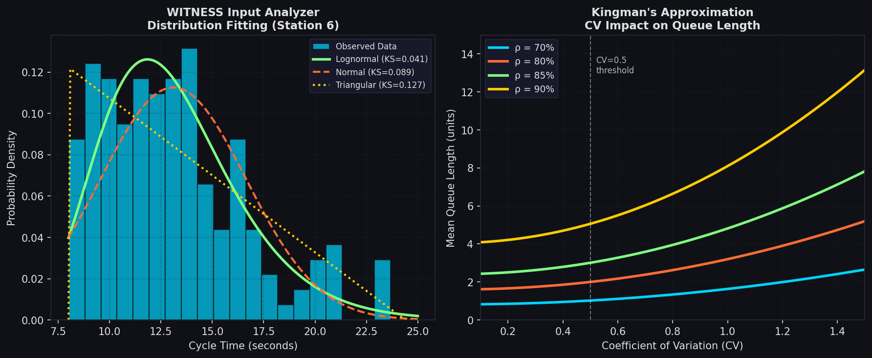
WITNESS Horizon includes a built-in Input Analyzer that fits statistical distributions to observed cycle-time samples. Import a CSV of time-study observations, and the tool ranks candidate distributions (normal, lognormal, Weibull, gamma) by chi-squared and Kolmogorov–Smirnov goodness-of-fit. The fitted distribution expression is then pasted directly into the Machine element's cycle-time field.
This step is critical: using a fixed mean instead of a fitted distribution typically underestimates queue lengths by 20–40% in lines with high coefficient of variation (CV > 0.5).
3. Run the Line-Balance Experiment
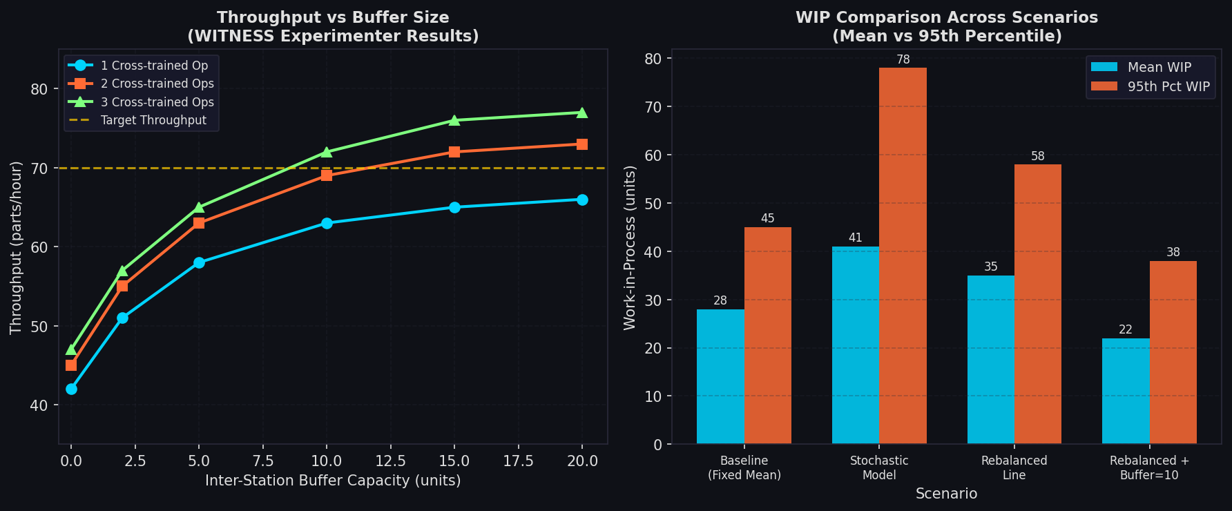
Once the baseline model is validated against historical throughput data, WITNESS Horizon's Experimenter module automates what-if scenarios. A typical line-balance experiment varies:
| Factor | Range |
|---|---|
| Station cycle time (±10%) | Operator pacing improvement |
| Buffer capacity | 0 to 20 units |
| Number of cross-trained operators | 1 to 4 |
| Shift pattern | 8 h single / 12 h rotating |
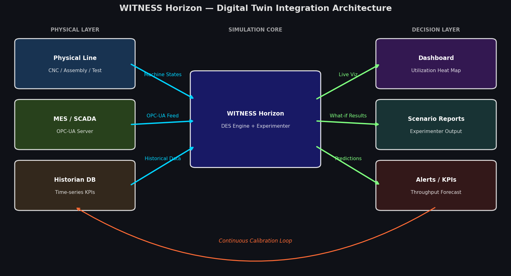
The Experimenter runs a full-factorial or Latin Hypercube design, collects KPIs (throughput, WIP, station utilization, lead time), and ranks scenarios by a user-defined objective function—for example, maximize throughput subject to WIP ≤ 50 units.
4. Interpret the Utilization Heat Map
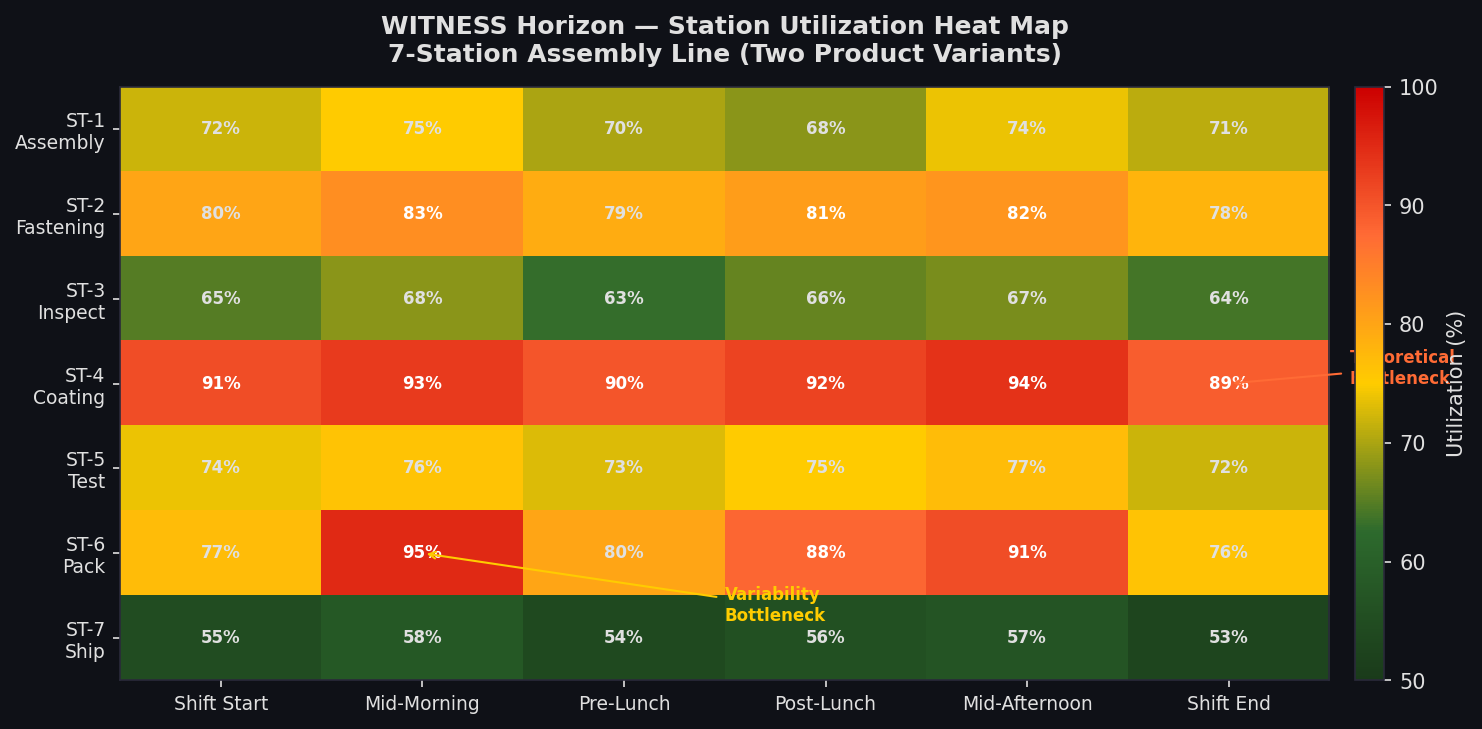
WITNESS Horizon's Dashboard renders a color-coded utilization heat map across all stations and time periods. Stations above 85% utilization are flagged as potential bottlenecks; stations below 60% are candidates for task reallocation or operator sharing. The heat map updates live during simulation runs, making it easy to spot transient bottlenecks that only appear during shift changeovers or after a machine failure.
A key insight from lean practice: the constraint in a stochastic line is rarely the station with the highest average utilization—it is often the station with the highest variability-adjusted load (utilization × CV²). WITNESS surfaces this metric in its advanced statistics panel.
Practical Results: A Case Study Pattern
In a representative automotive sub-assembly line with seven stations and two product variants, a WITNESS Horizon model revealed that the theoretical bottleneck (Station 4, 92% utilization) was not the actual throughput limiter. Station 6, at 78% utilization but with a CV of 1.3 due to frequent micro-stoppages, was generating a queue that propagated upstream and reduced effective throughput by 11%. Reallocating one task element from Station 6 to Station 5 (reducing Station 6's load to 68%) increased line throughput by 9% without any capital investment.
Integration with MES and Digital Twin Pipelines
WITNESS Horizon supports OPC-UA and REST API connectivity, enabling live data feeds from Manufacturing Execution Systems (MES). In a digital twin configuration, real-time machine state signals update the simulation's failure/repair distributions continuously, so the model's throughput predictions stay calibrated as the physical line ages. This closes the loop between the simulation model and the shop floor, turning a one-time analysis tool into a persistent operational decision-support system.
Key Takeaways
- Use fitted distributions, not fixed means: stochastic variability is the primary driver of queue formation and throughput loss in balanced lines.
- Variability-adjusted utilization (utilization × CV²) is a better bottleneck predictor than raw utilization alone.
- The Experimenter module automates scenario comparison, reducing analysis time from days to hours.
- OPC-UA integration enables continuous model calibration for digital twin applications.
- WITNESS Horizon's manufacturing object library accelerates model build time compared to general-purpose DES tools, making it practical for project timelines of two to four weeks.