MIKE FLOOD: Mastering 1D–2D Coupled Flood Simulation for Urban and Coastal Inundation Modeling
Urban flood modeling presents a fundamental challenge: floodwater simultaneously flows through underground drainage networks, open channels, and overland surfaces — each governed by different hydraulic regimes. DHI's MIKE FLOOD addresses this by tightly coupling one-dimensional (1D) and two-dimensional (2D) hydraulic solvers within a single simulation framework. For practitioners working on urban stormwater, coastal surge, or river-floodplain inundation, understanding MIKE FLOOD's coupling architecture and configuration options is essential to producing reliable, defensible results.
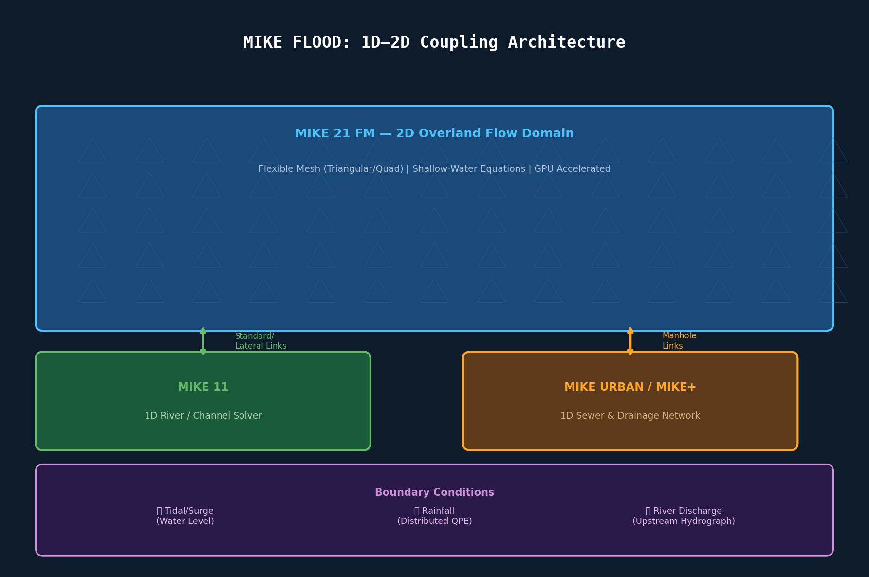
The 1D–2D Coupling Architecture
MIKE FLOOD integrates three core DHI engines:
- MIKE 11 — a 1D implicit finite-difference solver for rivers, channels, and pipe networks
- MIKE URBAN (or MIKE+ Drainage) — a 1D sewer and drainage network solver
- MIKE 21 — a 2D finite-volume shallow-water solver for overland and coastal flow
The coupling is bidirectional and dynamic: at each time step, water levels and discharges are exchanged across defined link structures. This means a surcharging sewer can inject flow onto the 2D surface domain, and rising floodwater on the surface can suppress further drainage outflow — a critical feedback loop that purely 1D or purely 2D models cannot capture.

Link Types and When to Use Them
MIKE FLOOD supports four coupling link types, each suited to different physical interfaces:
| Link Type | Use Case | Key Parameter |
|---|---|---|
| Standard Link | River channel ↔ floodplain | Lateral weir or structure |
| Lateral Link | Distributed exchange along a channel bank | Weir coefficient per cell |
| Structure Link | Culverts, gates, bridges | Structure geometry |
| Zero-Flow Link | Blocking boundaries | N/A |
For urban applications, Standard Links connecting MIKE URBAN manholes to MIKE 21 surface cells are the most common configuration. Each manhole is assigned a 2D cell; when the hydraulic grade line exceeds the manhole rim elevation, flow is transferred to the surface using a weir formula:
Q = C_d × L × (H_1D - H_2D)^(3/2)where C_d is the discharge coefficient (typically 0.5–0.8 for circular openings), L is the effective weir length, and the head difference drives the exchange direction.
Setting Up a Coupled Urban Flood Model
1. Domain Discretization
The 2D mesh resolution is the single largest driver of both accuracy and runtime. For urban areas, a flexible mesh (triangular/quadrilateral) with local refinement is strongly preferred over a uniform rectangular grid:
- Building footprints: 2–5 m cells to resolve flow paths between structures
- Street corridors: 3–8 m cells aligned with road geometry
- Open areas/parks: 10–20 m cells acceptable
DHI's MIKE Zero mesh generator supports polygon-based refinement zones. Import building footprints as hard boundaries (not just roughness zones) to force flow around structures rather than through them — this is a common source of underestimated peak depths in urban models.
2. Roughness Parameterization
Manning's n values should be assigned by land-use class using a GIS polygon overlay:
- Impervious surfaces (roads, rooftops): n = 0.011–0.015
- Grass/parks: n = 0.025–0.035
- Dense urban vegetation: n = 0.05–0.10
Avoid the temptation to use a single spatially uniform roughness — it will systematically bias flow velocities and inundation extents.
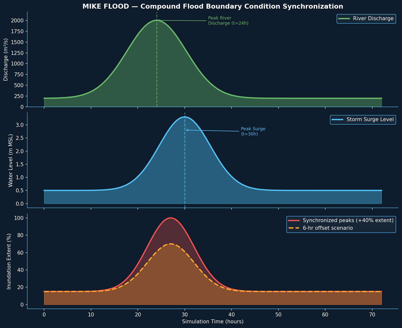
3. Boundary Conditions for Coastal–Fluvial Compound Events
For coastal cities, compound flooding (simultaneous riverine and tidal/surge forcing) requires careful boundary condition setup:
- Upstream river boundaries: Discharge hydrograph from a hydrological model (e.g., MIKE SHE or SWAT+)
- Coastal/tidal boundaries: Water level time series from a surge model (e.g., MIKE 21 HD or ADCIRC)
- Rainfall: Spatially distributed using a MIKE 21 rainfall source term, ideally from radar QPE or a downscaled NWP product
Synchronizing the timing of peak river discharge and peak surge is critical — a 6-hour offset between the two can change maximum inundation extent by 20–40% in low-lying coastal cities.
Performance Optimization: GPU Acceleration and Adaptive Time-Stepping
MIKE 21's flexible mesh solver supports GPU acceleration via NVIDIA CUDA, delivering 10–50× speedups over CPU-only runs for meshes exceeding ~500,000 elements. Key configuration settings in the MIKE 21 FM .m21fm file:
[GPU]
UseGPU = true
GPUDeviceID = 0
Pair GPU acceleration with adaptive time-stepping (CFL-based) to maintain numerical stability during rapid inundation fronts without over-constraining the time step during quiescent periods. Set a maximum CFL number of 0.8 and a minimum time step of 0.1 s for urban applications.
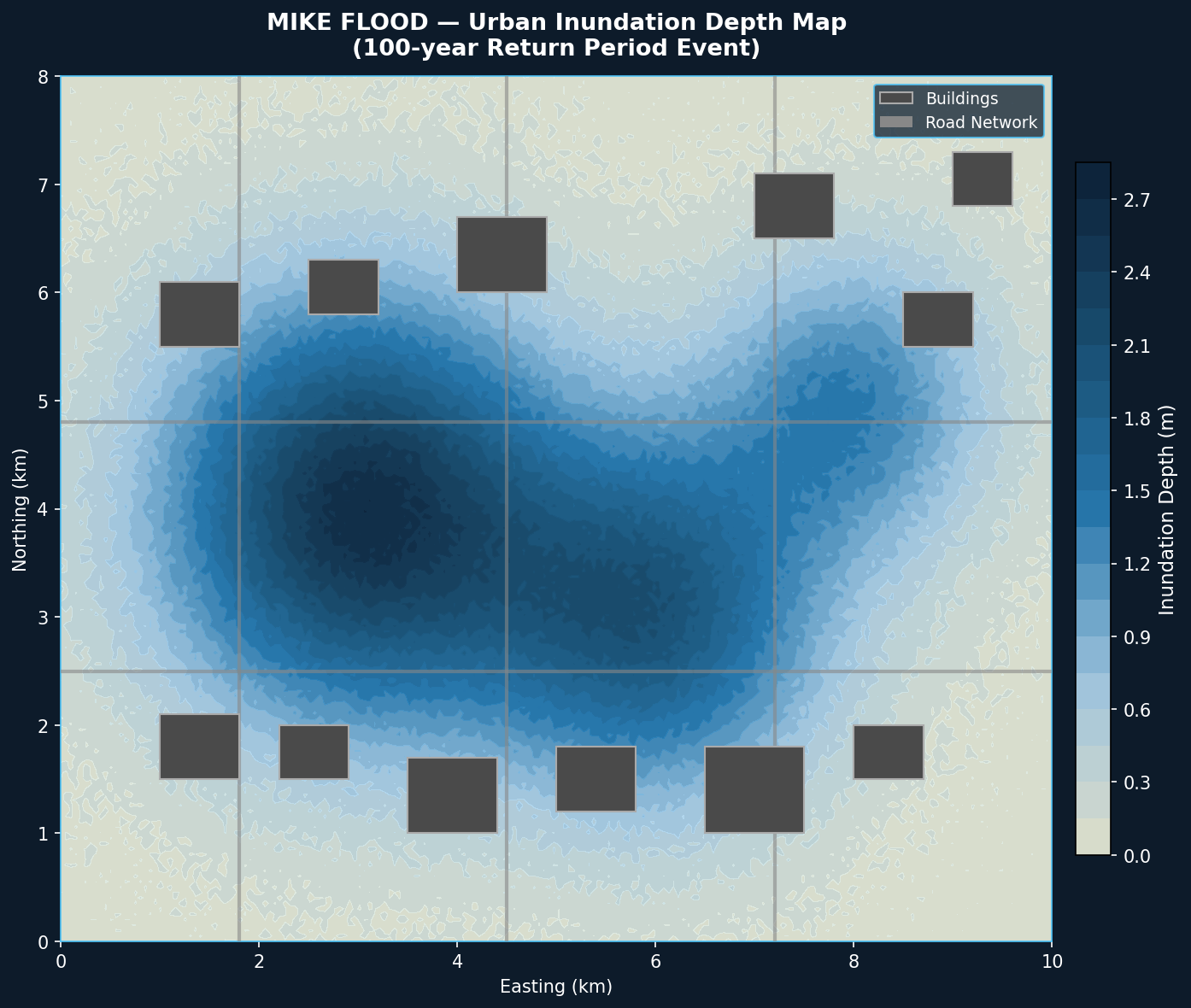
For ensemble runs (e.g., 100-year return period uncertainty analysis), DHI's MIKE Cloud platform enables parallel batch execution across cloud instances, reducing wall-clock time from days to hours.
Validation Best Practices
A coupled MIKE FLOOD model should be validated against at minimum two independent data sources:
- Flood extent polygons from post-event aerial/satellite imagery (e.g., Copernicus EMS, Sentinel-1 SAR) — use the Critical Success Index (CSI) metric, targeting CSI > 0.6 for urban areas
- Water level time series from stream gauges or temporary pressure transducers — target Nash-Sutcliffe Efficiency (NSE) > 0.7
Common calibration parameters are Manning's n (surface roughness), manhole discharge coefficients, and pipe roughness (Colebrook-White k_s). Avoid over-calibrating to a single event — always validate on a held-out event before operational deployment.
Integration with GIS and Post-Processing
MIKE FLOOD outputs (.dfs2 for 2D results, .res11 for 1D) can be exported to GeoTIFF or NetCDF for integration with QGIS, ArcGIS, or Python-based workflows. The mikeio Python library provides direct access to DHI result files:
import mikeio

ds = mikeio.open("flood_results.dfs2")
max_depth = ds["Water Depth"].max(axis=0)
max_depth.to_dataframe().to_csv("max_inundation_depth.csv")
This enables automated report generation, damage assessment integration (via depth-damage curves), and ingestion into early warning dashboards.
Summary
MIKE FLOOD's bidirectional 1D–2D coupling makes it one of the most physically rigorous tools available for urban and coastal flood simulation. The key to successful deployment lies in careful mesh design around buildings, appropriate link parameterization at drainage–surface interfaces, and compound boundary condition synchronization for coastal applications. With GPU acceleration and cloud-based ensemble capabilities, operational-scale probabilistic flood mapping is now tractable for city-scale domains.