
AgriSim Pro: Leveraging Monte Carlo Sensitivity Analysis for Robust Crop Yield Forecasting
Crop yield forecasting is inherently uncertain. Soil variability, unpredictable weather, pest pressure, and market-driven management decisions all introduce stochastic noise that deterministic simulation runs cannot capture. AgriSim Pro—a commercially supported extension of the APSIM (Agricultural Production Systems sIMulator) framework—addresses this limitation through a tightly integrated Monte Carlo sensitivity analysis (MCSA) engine. This article examines how to configure and interpret MCSA workflows in AgriSim Pro to produce statistically defensible yield forecasts for decision support.
Why Deterministic Runs Are Insufficient
A single APSIM simulation run uses fixed parameter values: a specific soil hydraulic conductivity, a single sowing date, one weather file. The output is a single yield number. In practice, every one of those inputs carries measurement uncertainty or natural variability. Running only the "best-estimate" scenario can mislead agronomists into false precision—reporting "6.2 t/ha wheat" when the defensible range is 4.8–7.6 t/ha.
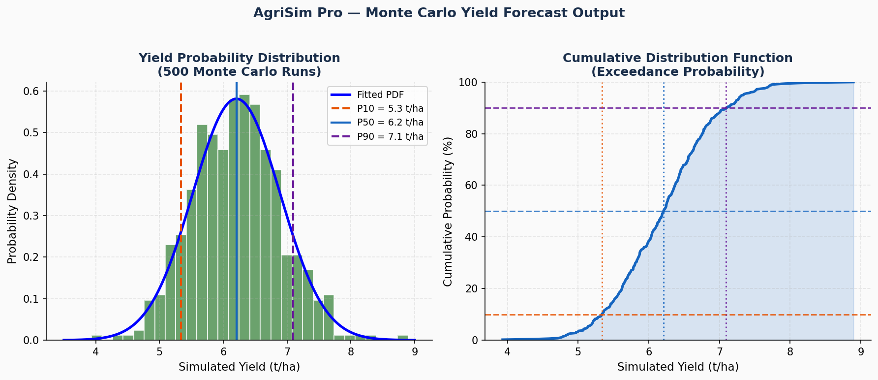
Monte Carlo analysis resolves this by sampling input parameters from probability distributions, running hundreds or thousands of simulations, and aggregating the resulting output distribution. The result is a probability density function (PDF) of yield outcomes, from which confidence intervals, value-at-risk metrics, and sensitivity rankings can be derived.
AgriSim Pro's MCSA Architecture
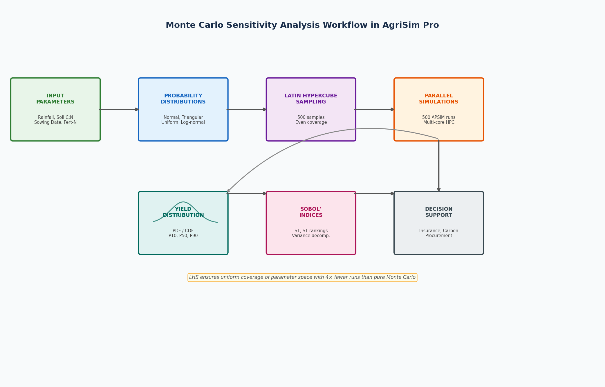
AgriSim Pro wraps the APSIM simulation kernel with a Python-based orchestration layer that handles:
- Parameter space definition – Users specify probability distributions (normal, log-normal, triangular, uniform, or empirical) for any APSIM input parameter via a YAML configuration file.
- Latin Hypercube Sampling (LHS) – Rather than pure random sampling, AgriSim Pro uses LHS to ensure even coverage of the parameter space with fewer runs. A 500-sample LHS design typically achieves convergence that would require 2,000+ pure Monte Carlo draws.
- Parallel execution – The orchestration layer distributes simulation runs across available CPU cores (or a SLURM HPC cluster) using Python's
multiprocessingmodule, reducing wall-clock time from hours to minutes. - Variance-based sensitivity indices – After runs complete, AgriSim Pro computes Sobol' first-order and total-effect indices to rank which input parameters drive the most output variance.
Configuring a Sensitivity Analysis Run
1. Define the Parameter Distributions
Create a sensitivity_config.yaml file in your project directory:
parameters:
  - name: SoilCN
    distribution: normal
    mean: 12.5
    std: 2.1
    bounds: [8, 20]
  - name: SowingDate
    distribution: uniform
    low: "2024-05-01"
    high: "2024-05-25"
  - name: FertN_kg_ha
    distribution: triangular
    low: 80
    mode: 120
    high: 160
  - name: RainfallScaleFactor
    distribution: normal
    mean: 1.0
    std: 0.12
    bounds: [0.6, 1.4]

outputs:
  - HarvestYield_t_ha
  - NitrogenLeaching_kg_ha

sampling:
  method: lhs
  n_samples: 500
  seed: 42
2. Run the Analysis
agrimsim-pro sensitivity \
  --config sensitivity_config.yaml \
  --apsim-file MyWheatPaddock.apsimx \
  --output-dir ./results/mc_run_01 \
  --cores 8
AgriSim Pro will generate 500 .apsimx variants, execute them in parallel, and write a results_summary.csv containing all input samples and corresponding outputs.
3. Interpret the Output
AgriSim Pro's built-in reporting module produces:
- Yield PDF and CDF plots – Visualize the probability of exceeding target yields (e.g., P90 yield for contract farming).
- Sobol' sensitivity bar chart – Identify which parameters (e.g., rainfall scaling vs. sowing date) contribute most to yield variance.
- Scatter plots – Detect non-linear relationships between individual parameters and yield.
Interpreting Sobol' Sensitivity Indices
The Sobol' total-effect index (S_Ti) measures the fraction of output variance attributable to a parameter, including all its interactions with other parameters. A typical result for a dryland wheat scenario might look like:
| Parameter | S1 (First-Order) | ST (Total Effect) |
|---|---|---|
| RainfallScaleFactor | 0.52 | 0.61 |
| SowingDate | 0.18 | 0.24 |
| FertN_kg_ha | 0.09 | 0.11 |
| SoilCN | 0.04 | 0.07 |
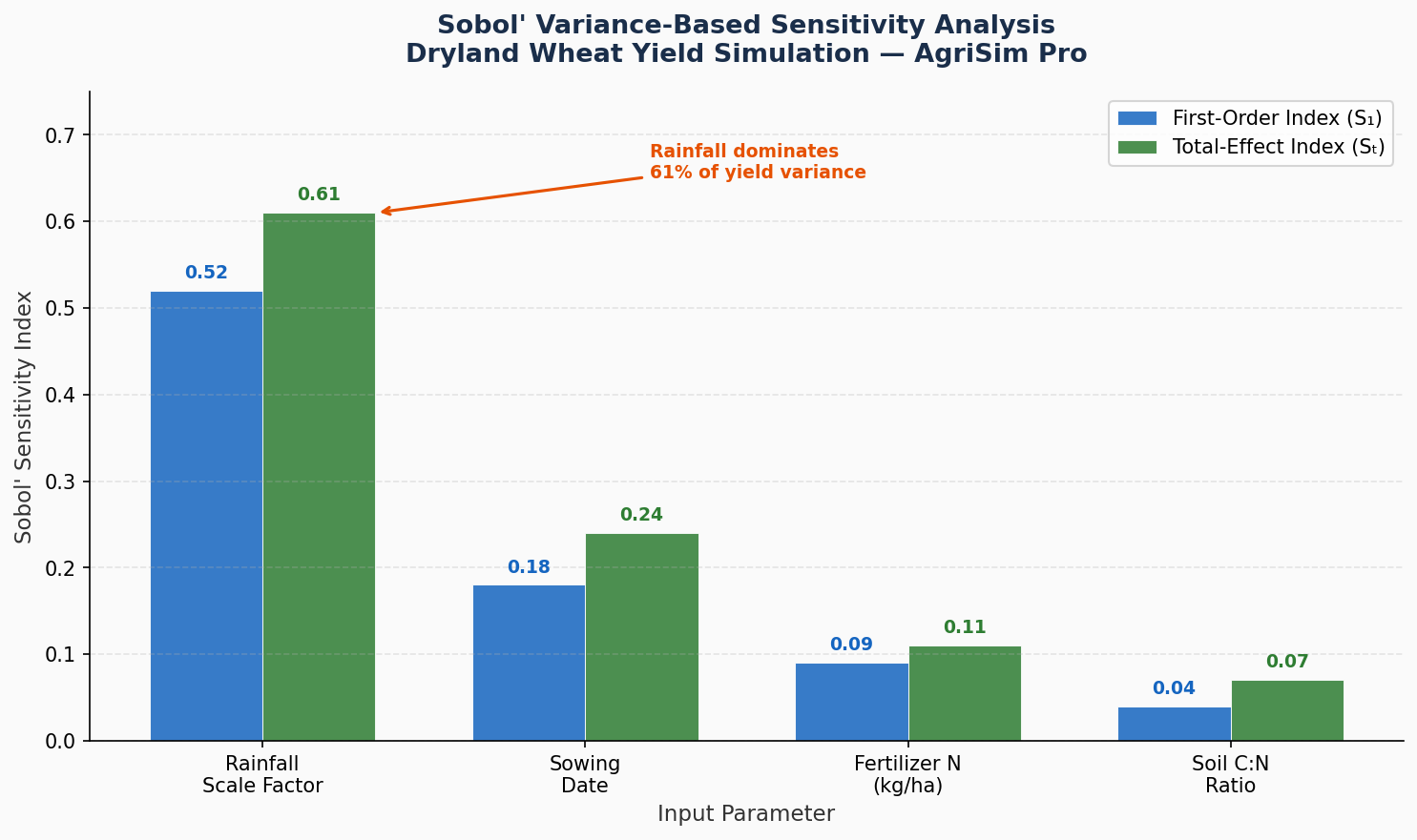
This table reveals that rainfall variability dominates yield uncertainty (61% of total variance), while soil carbon-to-nitrogen ratio has a minor effect. The practical implication: investing in better seasonal rainfall forecasts will reduce forecast uncertainty far more than improving soil characterization.
Best Practices
Bound your distributions carefully. Unbounded normal distributions can generate physically impossible parameter values (e.g., negative rainfall). Always set bounds in the YAML to clip samples to agronomically plausible ranges.
Validate with historical data before forecasting. Run the MCSA over historical years with known outcomes. If observed yields fall within the P10–P90 range in ≥80% of years, the uncertainty model is well-calibrated.
Separate aleatory from epistemic uncertainty. Weather variability is aleatory (irreducible); soil parameter uncertainty is epistemic (reducible with more sampling). Keeping these in separate sensitivity runs helps prioritize data collection investments.
Use ensemble weather files for climate scenarios. AgriSim Pro supports feeding multiple CMIP6 climate projections as the weather input distribution, enabling climate-risk-adjusted yield forecasts for 2030–2050 planning horizons.
Integration with Farm Management Decision Support
AgriSim Pro's MCSA outputs can be exported to JSON and consumed by farm management platforms (e.g., Trimble Ag Software, John Deere Operations Center) via REST API. The P10/P50/P90 yield estimates feed directly into:
- Input procurement planning – Order seed and fertilizer quantities aligned with the P50 scenario while maintaining buffer stock for the P90 upside.
- Crop insurance calibration – Actuaries use the yield PDF to set premium rates and trigger thresholds for parametric insurance products.
- Carbon credit verification – Probabilistic N-leaching estimates support conservative baseline calculations required by Verra and Gold Standard protocols.
Conclusion
Monte Carlo sensitivity analysis transforms APSIM-based crop simulation from a single-point estimate into a statistically rigorous decision-support tool. AgriSim Pro's LHS sampling, parallel execution, and Sobol' index reporting make this workflow accessible to agronomists without a statistics background. By quantifying which input uncertainties matter most, practitioners can focus data collection efforts where they will have the greatest impact on forecast quality—ultimately improving the reliability of yield forecasts for farm management, insurance, and climate adaptation planning.