Ecopath with Ecosim: Mass-Balance Ecosystem Modeling for Marine and Freshwater Fisheries Management

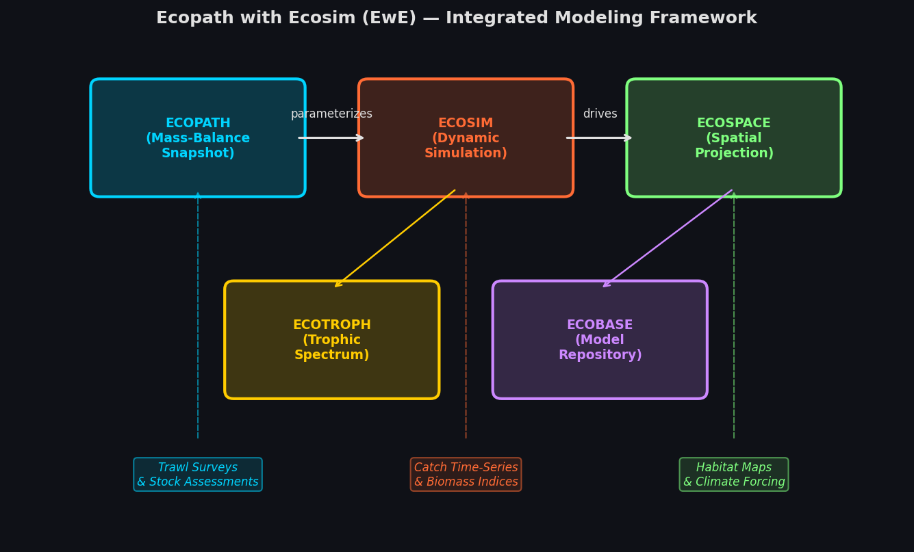
Ecopath with Ecosim (EwE) is the world's most widely used ecosystem modeling framework for aquatic systems, with over 700 published models spanning coral reefs, upwelling systems, large marine ecosystems, and freshwater lakes. Developed originally by Jeff Polovina at NOAA and later extended by Villy Christensen and Carl Walters at the University of British Columbia, EwE provides a trophic mass-balance platform that links static snapshots (Ecopath) with dynamic time-series simulations (Ecosim) and spatially explicit projections (Ecospace). For fisheries scientists, conservation managers, and climate impact analysts, EwE offers a uniquely integrated workflow that no single-species stock assessment tool can replicate.

The Ecopath Mass-Balance Core

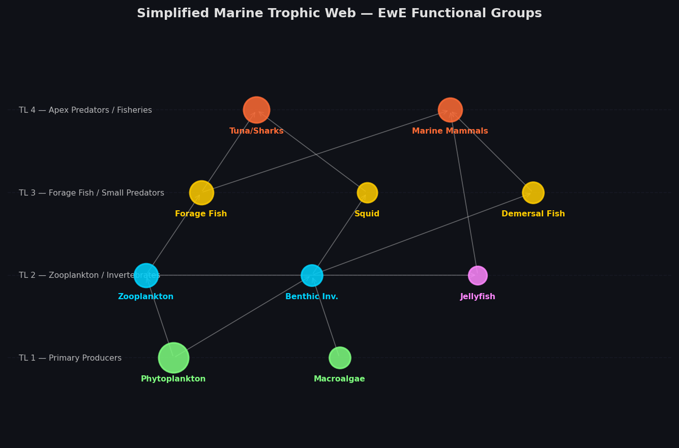
The foundation of every EwE model is the Ecopath module, which enforces a mass-balance constraint across all functional groups simultaneously:

Production = Predation mortality + Fishing mortality + Other mortality + Net migration

Each functional group — from phytoplankton to apex predators — is parameterized with:

• B (biomass, t km⁻²)
• P/B (production-to-biomass ratio, yr⁻¹, equivalent to total mortality Z for most groups)
• Q/B (consumption-to-biomass ratio, yr⁻¹)
• EE (ecotrophic efficiency, the fraction of production consumed within the system)
• Diet matrix (DC, fraction of each predator's diet from each prey group)

EwE solves the linear system to estimate any single unknown per group, making it possible to build a balanced model even when empirical data are sparse. The Pedigree module assigns confidence scores to each input, propagating uncertainty into downstream analyses. A well-balanced Ecopath model typically achieves EE < 1 for all groups and realistic trophic levels (TL) that match independent estimates from stable isotope studies.

Ecosim: Dynamic Simulation with Foraging Arena Theory

Ecosim extends the static Ecopath snapshot into time-dynamic simulations using the foraging arena concept. Prey biomass is partitioned into a vulnerable fraction (accessible to predators) and an invulnerable fraction (in refugia). The vulnerability parameter (v) controls predator–prey interaction strength:

• v → 1: bottom-up control (prey-limited dynamics)
• v → ∞: top-down control (predator-limited, Lotka-Volterra-like)
• v ≈ 2: mixed control (default starting point)

Fitting v values to observed time-series data (catch, biomass indices from surveys) is the critical calibration step. Ecosim's time-series fitting routine minimizes a weighted sum-of-squares objective across all groups simultaneously, using a gradient-based optimizer. Analysts typically run sensitivity analyses across v-space to identify which predator–prey pairs drive model uncertainty.

Fishing Policy Optimization

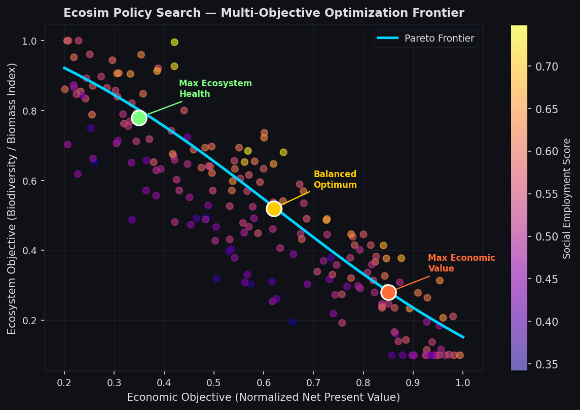
Ecosim's Policy Search module allows managers to optimize fishing mortality rates (F) across fleets to maximize a multi-criteria objective function combining:

1. Economic value (landed value minus costs)
2. Social employment (crew-days weighted by fleet)
3. Ecosystem structure (mandated biomass targets for protected species)
4. Biodiversity (Shannon diversity index of the catch)

The optimizer uses a quasi-Newton algorithm over a 20–50 year projection horizon. A typical workflow for a Pacific groundfish system might constrain rockfish biomass to ≥ 40% of unfished B₀ while maximizing net present value of the trawl and longline fleets — a multi-objective problem that single-species MSY frameworks cannot address.

Ecospace: Spatially Explicit Projections

Ecospace maps Ecosim dynamics onto a 2-D grid, allowing analysts to evaluate:

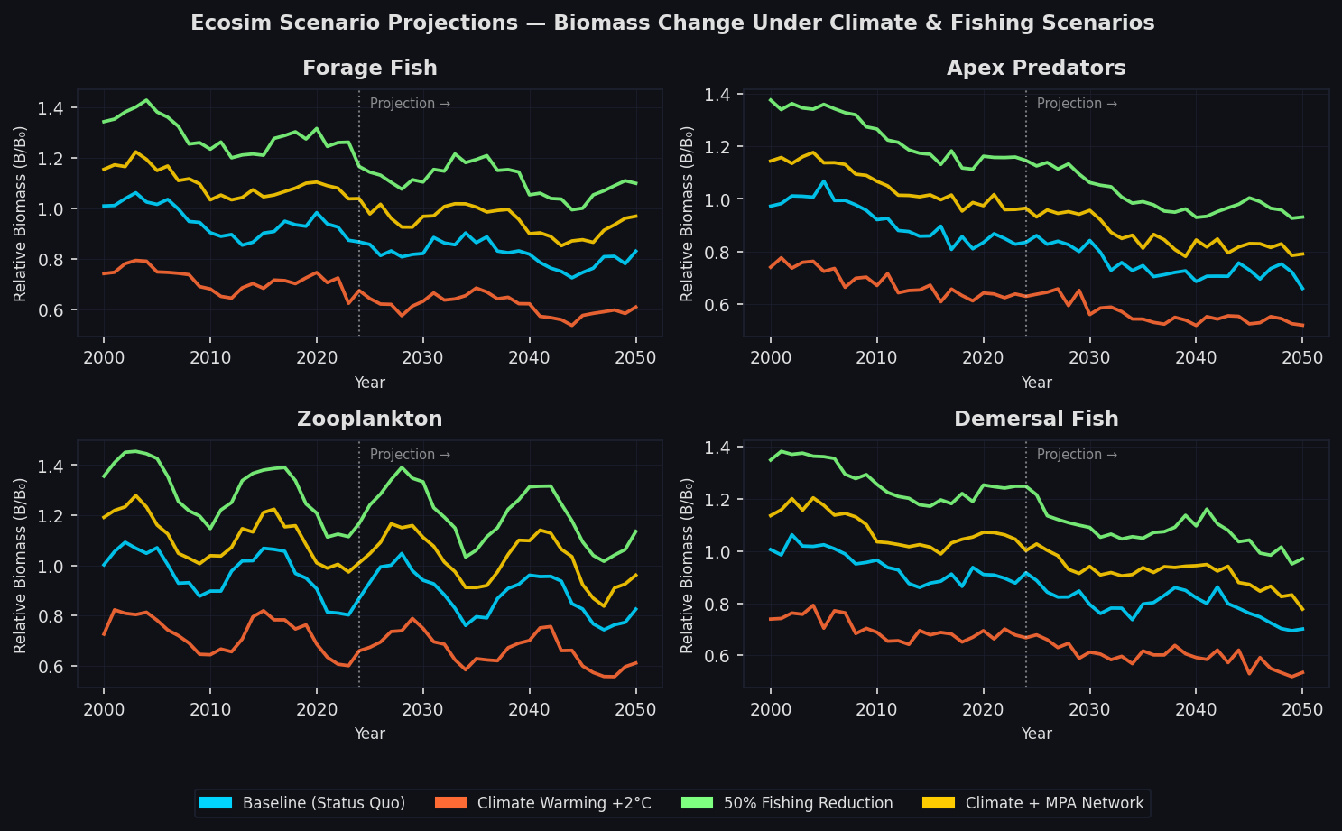
• Marine Protected Area (MPA) design: comparing no-take zones, partial closures, and seasonal restrictions
• Habitat forcing: linking benthic habitat maps (seagrass, coral, soft sediment) to group-specific carrying capacities
• Climate-driven range shifts: coupling sea surface temperature (SST) and dissolved oxygen projections from ROMS or NEMO to habitat suitability functions

Ecospace integrates with Atlantis (CSIRO's end-to-end model) and can ingest NetCDF forcing fields directly, making it compatible with CMIP6 climate projections. Spatial resolution is typically 5–25 km for regional models, with finer grids (1–2 km) used for estuarine or reef-scale applications.

Practical Workflow: Building a Shelf Ecosystem Model

A standard EwE project for a continental shelf system follows these stages:

1. Define functional groups (20–50 groups is typical): aggregate species by trophic role, life stage, and data availability
2. Parameterize Ecopath: compile biomass estimates from trawl surveys, P/B from stock assessments, Q/B from bioenergetics literature, diet from stomach content studies
3. Balance the model: iterate on EE values, check for unrealistic predation mortalities, use the Ecopath wizard for automated balancing
4. Load time-series: import annual catch and biomass index data (1980–present is typical)
5. Fit Ecosim: run the vulnerability search, assess SS improvement, validate against withheld data
6. Run scenarios: climate forcing (SST, primary production anomalies), fishing effort changes, MPA configurations
7. Ecospace projection: map spatial outcomes, generate heat maps of biomass change under each scenario

Integration with Climate and Biogeochemical Models

EwE's Ecotroph plugin implements a trophic spectrum approach that couples directly to primary production outputs from biogeochemical models (e.g., PISCES, COBALT, MEDUSA). Rather than resolving individual species, Ecotroph distributes production across trophic levels using a transfer efficiency function, enabling rapid screening of climate scenarios across large marine ecosystems where full species-resolved models are computationally prohibitive.

For higher-resolution coupling, the EwE–ROMS framework links Ecospace to the Regional Ocean Modeling System, with ROMS providing physical transport (advection, diffusion) for plankton groups while EwE handles the upper trophic level dynamics. This two-way coupling has been applied to the California Current, the North Sea, and the Benguela upwelling system.

Strengths, Limitations, and Best Practices

Strengths:

• Handles data-poor situations through mass-balance constraints
• Integrates fishing economics, ecology, and spatial management in one framework
• Large global community with shared model databases (EcoBase, >500 published models)
• Free, open-source (GPL), with active development at the Institute for the Oceans and Fisheries, UBC

Limitations:

• Steady-state Ecopath assumption may not hold in rapidly changing systems
• Vulnerability parameters are difficult to estimate independently; overfitting risk in Ecosim calibration
• Ecospace spatial resolution is coarser than dedicated hydrodynamic models
• No explicit age structure within functional groups (use Ecosim's multi-stanza feature for key species)

Best practices:

• Always run a Pedigree analysis before publishing; models with mean pedigree index < 0.4 should be treated as exploratory
• Use Monte Carlo uncertainty analysis (built into EwE 6.6+) to propagate parameter uncertainty into scenario outputs
• Validate Ecosim fits with a hindcast split: fit to 1980–2005, validate against 2006–2020 observations
• Document diet matrix sources explicitly; diet is the single largest source of structural uncertainty

Getting Started

EwE 6.6 runs on Windows (64-bit) and is freely available at ecopath.org. The EcoBase repository at ecobase.ecopath.org provides over 500 published models as starting templates. The UBC Fisheries Centre offers annual training workshops, and the EwE User Guide (Christensen et al., 2008) remains the definitive reference. For Python-based scripting of EwE outputs, the pyEwE package provides post-processing utilities for batch scenario analysis.

For marine ecosystem managers, climate impact analysts, and fisheries scientists, EwE provides an unmatched combination of ecological rigor, policy relevance, and community support — making it the essential starting point for any ecosystem-level simulation study.