

FESOM2: Unstructured-Mesh Ocean–Sea-Ice Simulation for Multi-Scale Climate Modeling
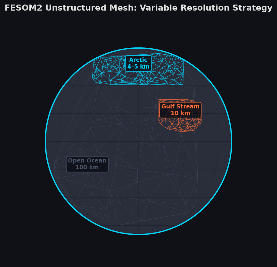
The ocean is not uniform. Narrow straits, continental shelves, ice-shelf cavities, and energetic boundary currents demand spatial resolution that structured-grid ocean models struggle to provide without prohibitive computational cost. FESOM2 (Finite Element Sea-ice Ocean Model, version 2) addresses this challenge with a fully unstructured triangular mesh that allows resolution to vary continuously from ~5 km in dynamically active regions to ~150 km in the open ocean — all within a single, globally consistent simulation.
Developed at the Alfred Wegener Institute (AWI) and released as open-source software, FESOM2 has become a cornerstone of the AWI Climate Model (AWI-CM) used in CMIP6 projections and is increasingly adopted by research groups worldwide for high-resolution process studies and decadal climate predictions.
Why Unstructured Meshes Matter for Ocean Modeling
Traditional structured-grid models (MOM6, NEMO, POP) use regular latitude–longitude or curvilinear grids. Achieving 1/12° resolution globally requires ~2 billion ocean cells and enormous memory bandwidth. FESOM2's unstructured approach lets modelers concentrate resolution exactly where it is needed:

- Arctic Ocean and sea-ice margins — resolving polynyas, leads, and ice-shelf melt cavities
- Western boundary currents (Gulf Stream, Kuroshio) — capturing mesoscale eddies that drive poleward heat transport
- Marginal seas and straits (Bering Strait, Denmark Strait) — correctly representing inter-basin exchange
- Coastal zones — bridging the gap between regional and global models without nesting
A mesh with 1.3 million surface nodes can simultaneously resolve the Arctic at 4.5 km and the central Pacific at 100 km, achieving effective global coverage at a fraction of the cost of a uniformly fine structured grid.
Core Architecture and Numerical Scheme
FESOM2 is written in Fortran 90/95 with MPI parallelism and scales efficiently to thousands of cores. Key numerical choices include:
- Finite-volume discretization on unstructured triangular prisms — the shift from FESOM1's finite-element formulation to a finite-volume approach in FESOM2 improved computational efficiency by roughly 3–5× while retaining mesh flexibility.
- Arbitrary Lagrangian–Eulerian (ALE) vertical coordinate — supports z*, σ, and hybrid vertical coordinates, enabling accurate representation of bottom topography and surface waves.
- Flux-corrected transport (FCT) tracer advection — monotone, mass-conserving advection that prevents spurious oscillations near sharp fronts.
- Sea-ice dynamics via EVP rheology — the elastic–viscous–plastic (EVP) solver handles sea-ice stress with sub-cycling, compatible with the unstructured mesh.
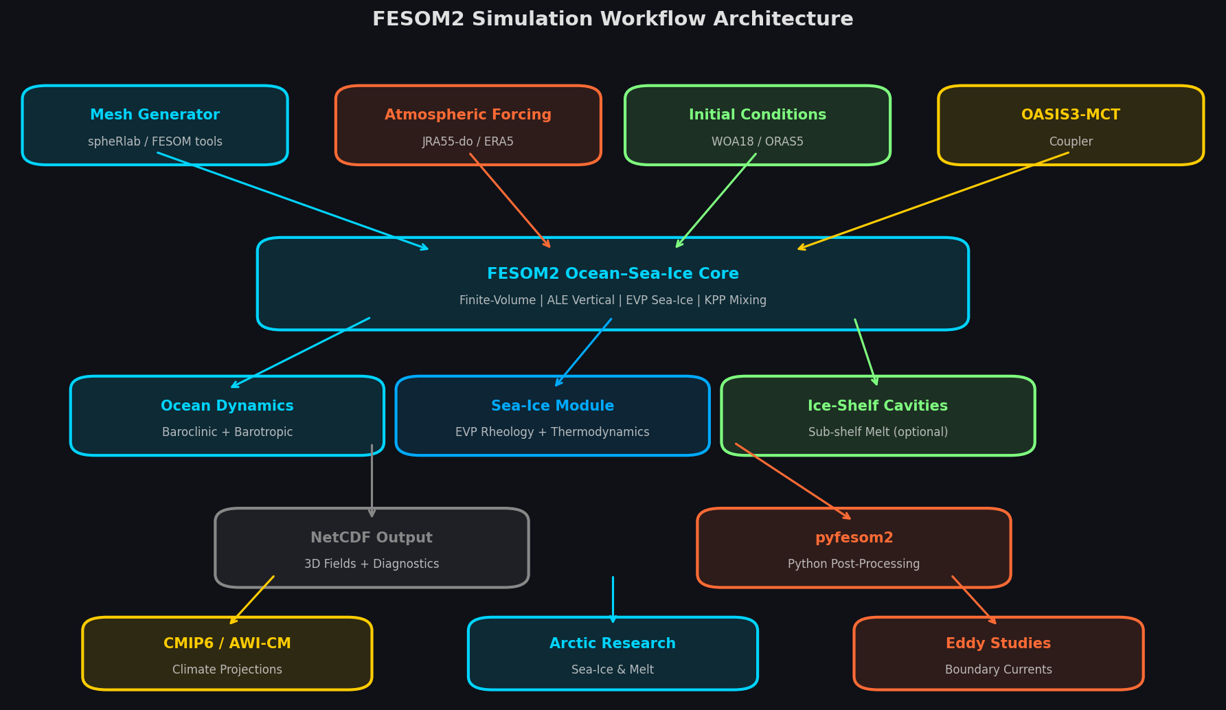
The model couples to the OASIS3-MCT coupler for integration into full Earth system models, and to the PISM ice-sheet model for ice-sheet–ocean interaction studies.
Setting Up a FESOM2 Simulation
Mesh Generation
Mesh generation is handled by the FESOM mesh generator (or the community tool spheRlab). A typical workflow:
# Example: define resolution zones in a mesh configuration
resolution_zones = {
    "arctic":    {"lon": [-180, 180], "lat": [65, 90],  "res_km": 5},
    "gulf_stream": {"lon": [-85, -30], "lat": [25, 50], "res_km": 10},
    "global":    {"res_km": 100}
}
The mesh generator produces nod2d.out, elem2d.out, and aux3d.out files that define node coordinates, element connectivity, and vertical layer structure. Mesh quality is assessed with the mesh_quality diagnostic before committing to a long run.
Namelist Configuration
FESOM2 uses a Fortran namelist (namelist.config) for runtime parameters:
&geometry
  cartesian = .false.
  fplane    = .false.
/
&calendar
  run_length    = 10        ! years
  run_length_unit = 'y'
  restart_length = 1
  restart_length_unit = 'y'
/
&physics
  use_ice = .true.
  use_cavity = .false.      ! set .true. for ice-shelf cavities
  mix_scheme = 'KPP'        ! KPP or PP vertical mixing
/
Atmospheric forcing is provided via CORE-II, JRA55-do, or ERA5 bulk formulae. The fesom.clock file tracks simulation time and restart state.
Running and Scaling
FESOM2 scales near-linearly to ~10,000 MPI tasks on modern HPC systems. A typical production run on a 1.3M-node mesh uses 960–1920 cores. The model outputs NetCDF files partitioned by MPI rank; the pyfesom2 Python library provides post-processing utilities:
import pyfesom2 as pf

mesh = pf.load_mesh('/path/to/mesh/')
temp = pf.get_data('/path/to/output/', mesh, 'temp', years=range(2000, 2010))
pf.plot(mesh, temp.mean('time'), cmap='RdBu_r', levels=20)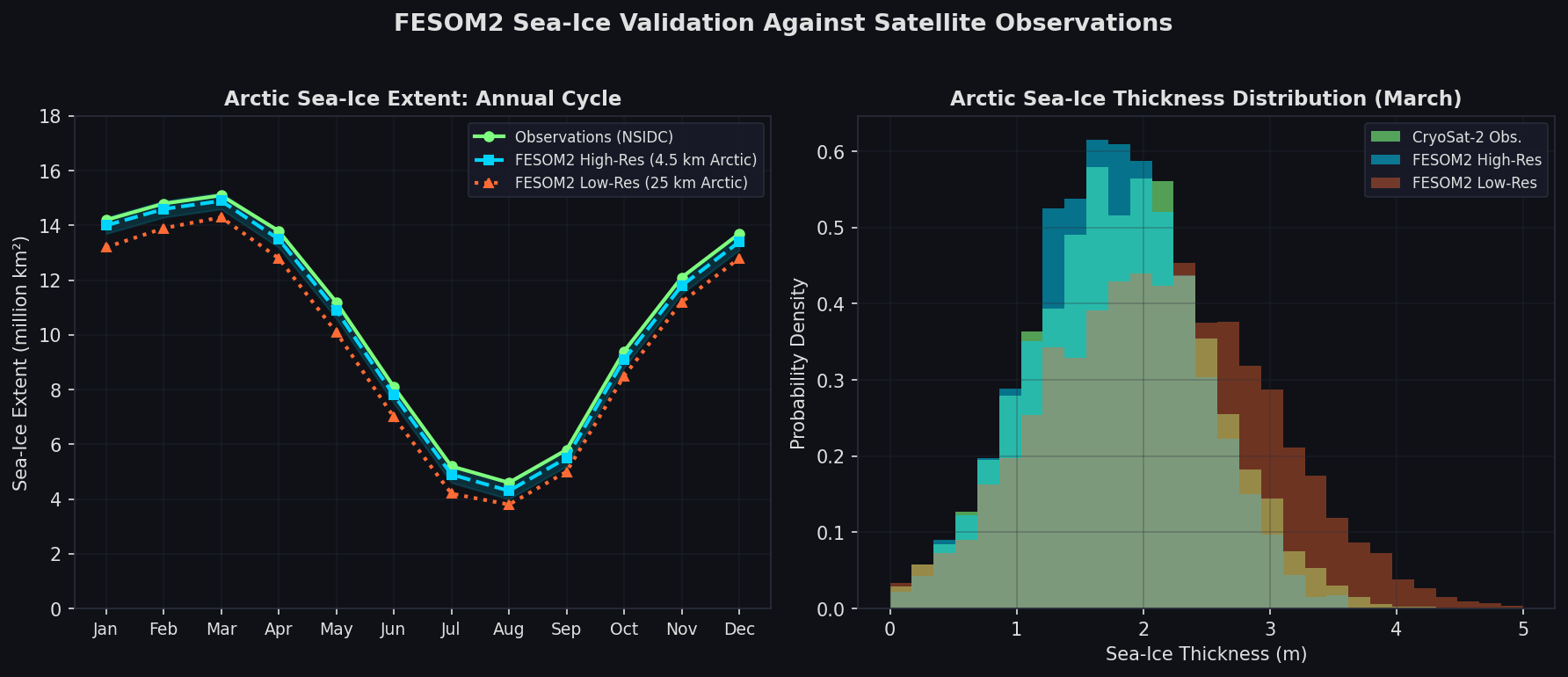
Key Capabilities for Climate Research
Multi-Resolution Sea-Ice Modeling
FESOM2's unstructured mesh is particularly powerful for Arctic sea-ice studies. By refining to 4–5 km in the Arctic while keeping coarser resolution elsewhere, simulations capture:
- Melt pond dynamics and their albedo feedback
- Sea-ice thickness distribution across the marginal ice zone
- Polynya formation driven by katabatic winds and ocean heat flux
Comparisons with ICESat-2 and CryoSat-2 altimetry show that high-resolution FESOM2 configurations reproduce observed sea-ice thickness gradients significantly better than coarser structured-grid models.
Mesoscale Eddy Permitting Simulations
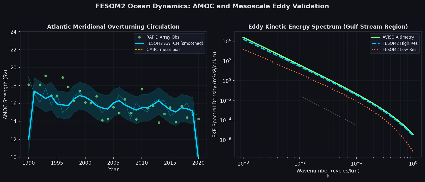
At 1/10° effective resolution in eddy-active regions, FESOM2 resolves the mesoscale eddy field that drives ~50% of poleward ocean heat transport. The model's eddy kinetic energy (EKE) spectra match satellite altimetry observations (AVISO/CMEMS) in both magnitude and spectral slope, validating the mesh refinement strategy.
Ice-Shelf Cavity Circulation
With use_cavity = .true., FESOM2 simulates sub-ice-shelf circulation beneath Antarctic ice shelves (Pine Island, Thwaites, Filchner-Ronne). This is critical for projecting basal melt rates that drive sea-level rise. The model resolves the ice pump mechanism — cold, fresh meltwater rising along the ice base and driving overturning circulation within the cavity.
Integration with AWI-CM and CMIP6
FESOM2 forms the ocean–sea-ice component of AWI-CM-1-1-MR, one of the CMIP6 models. In CMIP6 historical simulations, AWI-CM-1-1-MR demonstrated:
- Improved representation of the Atlantic Meridional Overturning Circulation (AMOC) compared to CMIP5 predecessors
- Realistic Arctic sea-ice extent trends over 1979–2014
- Reduced warm bias in the Southern Ocean, attributed to better eddy representation
Results are archived on the ESGF (Earth System Grid Federation) and accessible via the intake-esm Python catalog.
Practical Considerations
| Aspect | Guidance |
|---|---|
| Mesh resolution | Start with a coarse global mesh (~1M nodes) for spin-up; refine regionally for production |
| Spin-up | 200–500 years from climatological initial conditions (WOA18) for deep-ocean equilibration |
| Forcing | JRA55-do v1.5 recommended for historical simulations; OMIP-2 protocol for model intercomparison |
| Storage | ~500 GB/year for standard 3D output at 5-day frequency on a 1.3M-node mesh |
| Validation | Use pyfesom2 with Argo float climatologies, RAPID AMOC array data, and NSIDC sea-ice indices |
Further Resources
- FESOM2 GitHub Repository — source code, documentation, and issue tracker
- AWI-CM Model Description (Geosci. Model Dev.) — peer-reviewed model description paper
- pyfesom2 Documentation — Python post-processing toolkit
- FESOM Community Forum — mesh generation tips and configuration examples
- CMIP6 AWI-CM Data — ESGF data portal for model output
FESOM2 represents a significant advance in ocean climate modeling, enabling seamless multi-scale simulations that were previously impossible with structured-grid approaches. For research groups studying Arctic change, ice-shelf dynamics, or regional ocean–climate interactions, its unstructured mesh framework offers a compelling combination of physical fidelity and computational efficiency.