

AERMOD: Regulatory Air Dispersion Modeling for Industrial Source Impact Assessment
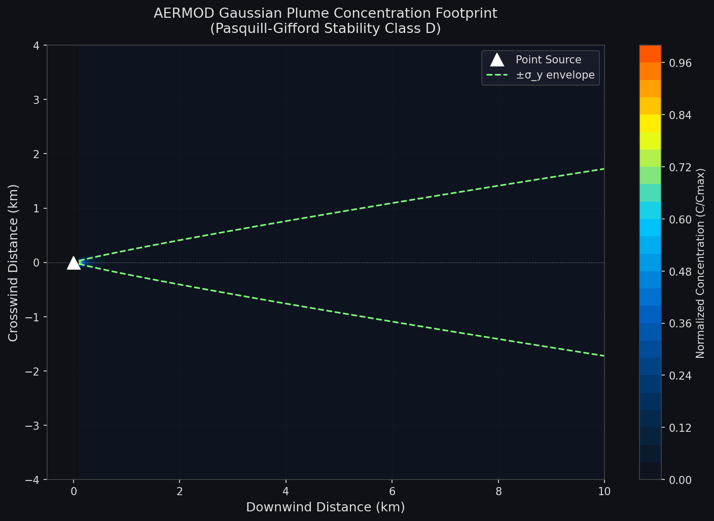
Air quality regulators and environmental engineers rely on accurate dispersion models to predict how pollutants travel from industrial stacks, area sources, and volume sources to nearby receptors. AERMOD (AMS/EPA Regulatory Model) is the U.S. Environmental Protection Agency's preferred steady-state Gaussian plume model for near-field dispersion in the planetary boundary layer (PBL). Since its adoption as the EPA's preferred model in 2005 (40 CFR Part 51, Appendix W), AERMOD has become the de facto standard for permit applications, National Ambient Air Quality Standards (NAAQS) compliance demonstrations, and Environmental Impact Assessments worldwide.
This article focuses on AERMOD's meteorological pre-processing pipeline, terrain handling, and building downwash algorithms—the three areas where practitioners most frequently encounter configuration pitfalls.
The AERMOD Modeling System Architecture
AERMOD is not a single executable but a tightly coupled three-component system:

| Component | Role |
|---|---|
| AERMET | Meteorological pre-processor: converts NWS surface and upper-air observations (or on-site data) into boundary-layer parameters (u*, L, zi, σv, σw) |
| AERMAP | Terrain pre-processor: ingests USGS Digital Elevation Model (DEM) data to compute receptor elevations and hill-height scales (hc) |
| AERMOD | Dispersion kernel: applies convective and stable PBL formulations, building downwash (PRIME algorithm), and dry/wet deposition |
The separation of pre-processing from dispersion calculation is intentional: AERMET and AERMAP outputs are reusable across multiple AERMOD runs with different source configurations, saving significant computation time during sensitivity analyses.
AERMET: Getting the Meteorology Right
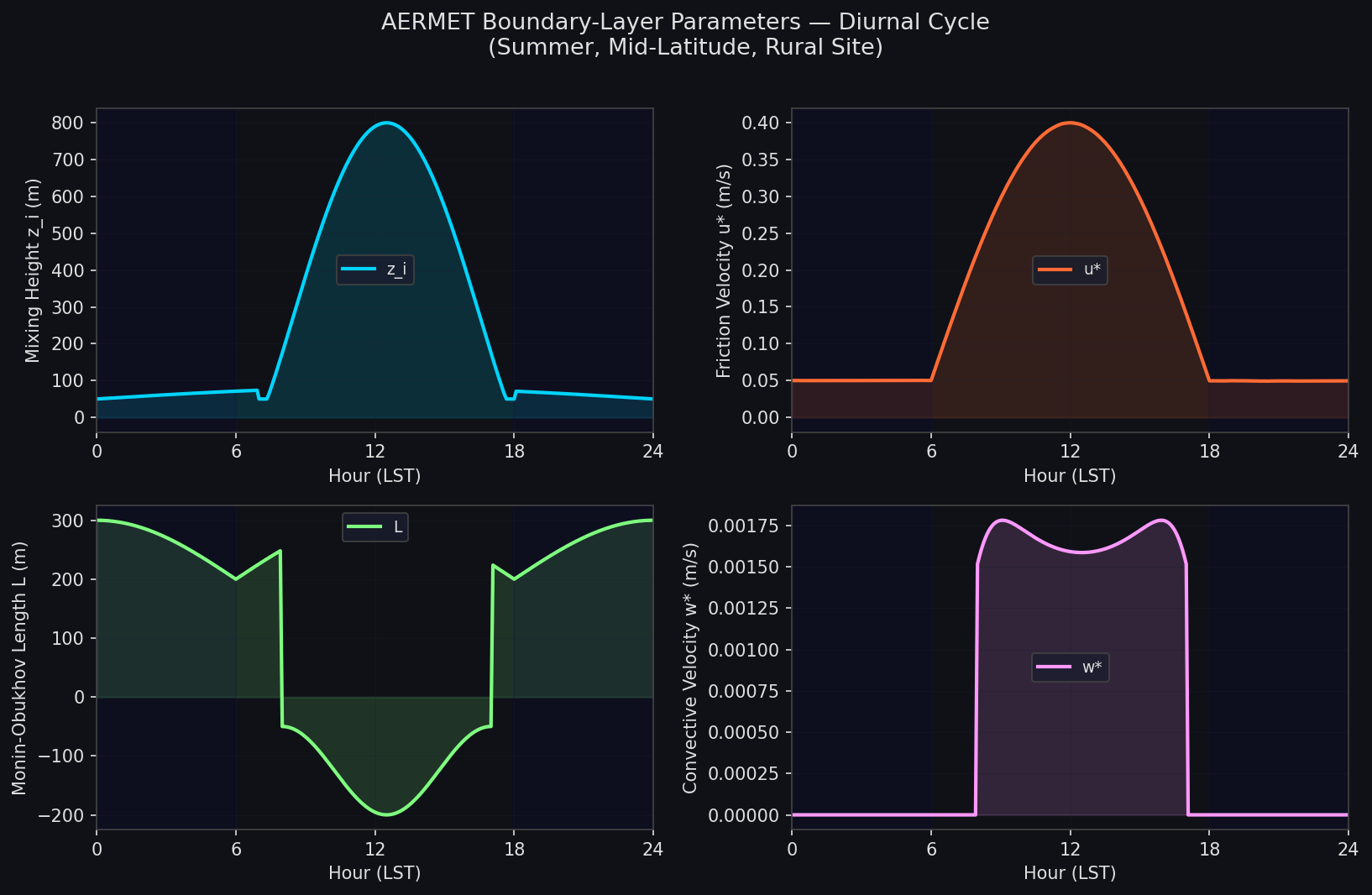
The most common source of AERMOD errors is improper AERMET configuration. AERMET requires two data streams:
- Surface observations (NWS ASOS/AWOS or on-site): wind speed/direction, temperature, cloud cover, ceiling height
- Upper-air soundings (NWS radiosonde, typically twice daily): temperature and wind profiles up to ~10 km
Stage 1–3 Processing
AERMET operates in three stages:
- Stage 1: Quality-assures and archives raw meteorological data
- Stage 2: Merges surface and upper-air data into a single merged file
- Stage 3: Estimates PBL parameters using the van Ulden–Holtslag similarity relationships
A critical Stage 3 parameter is the surface roughness length (z₀). AERMET requires a sector-averaged z₀ for each of 12 wind direction sectors. Underestimating z₀ in urban settings (e.g., using 0.03 m for open terrain instead of 0.5–1.0 m for dense urban) leads to overestimated mixing heights and underestimated ground-level concentrations—a non-conservative error in regulatory contexts.
On-Site vs. NWS Data
When a facility is located more than 50 km from the nearest NWS station, or when local terrain significantly influences wind patterns, on-site meteorological data is preferred. AERMET accepts 1-minute ASOS data or continuous on-site measurements. The EPA's AERMET User's Guide (EPA-454/B-03-002) provides detailed guidance on data substitution thresholds and representativeness criteria.
AERMAP: Terrain Influence on Plume Behavior
AERMOD uses a dual-plume formulation to handle complex terrain:
- Terrain-following state (S = 1): the plume follows the terrain surface
- Horizontal state (S = 0): the plume remains at its release height above mean sea level
The actual concentration is a weighted combination: C = f·C(S=1) + (1-f)·C(S=0), where the weighting factor f depends on the Froude number and the hill-height scale hc computed by AERMAP.
AERMAP ingests 1-arc-second (≈30 m) or 1/3-arc-second (≈10 m) National Elevation Dataset (NED) tiles. For receptors within 50 km of a source, the 1/3-arc-second DEM is strongly recommended—coarser terrain data can misrepresent ridge heights by tens of meters, directly affecting the hc calculation and the plume impaction probability.
Practical tip: Always verify AERMAP receptor elevations against field survey data for the 10–20 receptors nearest to the source. Elevation errors of ±5 m can shift predicted maximum concentrations by 15–30% in hilly terrain.
Building Downwash: The PRIME Algorithm
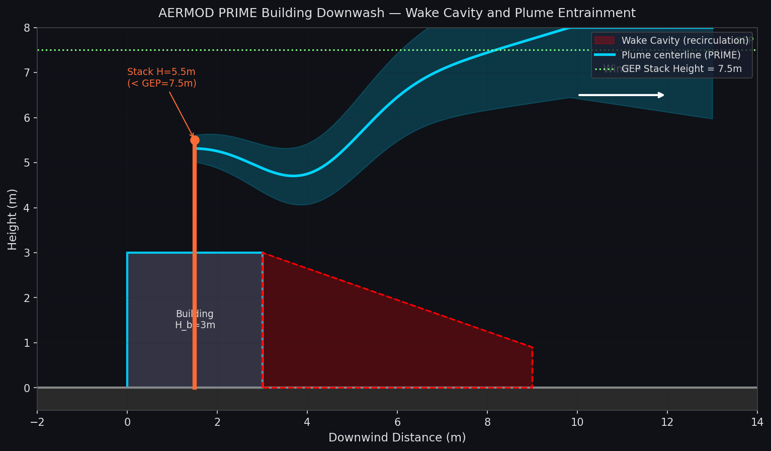
When a stack is shorter than 2.5 times the height of adjacent structures, the plume can be entrained into the building wake—a phenomenon called building downwash. AERMOD implements the PRIME (Plume Rise Model Enhancements) algorithm, which accounts for:
- Wake cavity recirculation: near-field zone of high turbulence immediately downwind of the building
- Streamline deflection: the plume trajectory is bent toward the ground as it passes over the building roof
- Enhanced dispersion: turbulence generated by the building increases σy and σz within the wake
To activate PRIME, the AERMOD input file must include a BUILDHGT keyword specifying building dimensions for each source. The BPIPPRM (Building Profile Input Program) utility automates the calculation of the projected building dimensions for each wind direction sector—a step that is frequently skipped, leading to underestimated downwash impacts.
For stacks subject to downwash, the Good Engineering Practice (GEP) stack height formula provides a minimum stack height to avoid entrainment: H_GEP = H_b + 1.5 × L, where H_b is the building height and L is the lesser of the building height or projected width. Stacks below GEP height require PRIME modeling regardless of permit requirements.
Receptor Grid Design
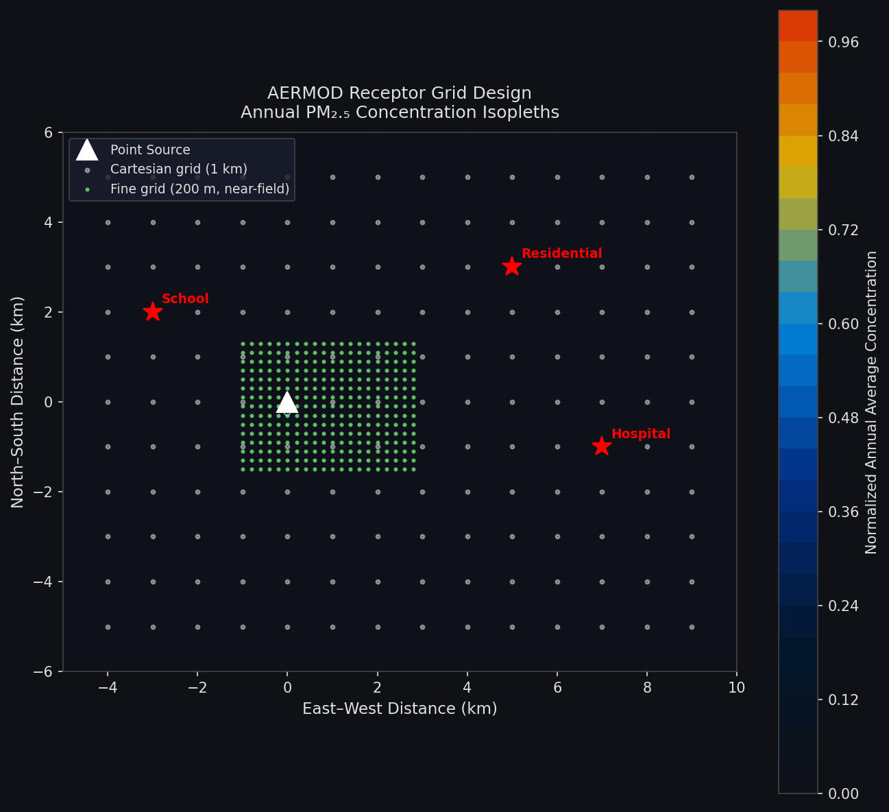
Receptor placement strategy significantly affects both the accuracy of predicted maximum concentrations and the computational cost of a run:
- Cartesian grid: uniform spacing (e.g., 100 m × 100 m) out to 5 km; increase to 500 m beyond 5 km
- Polar grid: concentric rings centered on the source; efficient for isolated point sources
- Discrete receptors: fence-line monitors, sensitive receptors (schools, hospitals), and property boundaries
For NAAQS compliance demonstrations, the EPA requires that the receptor grid be fine enough to capture the predicted maximum—typically ≤50 m spacing within 1 km of the source for PM₂.₅ and NO₂ analyses.
Post-Processing and Visualization
AERMOD output files (.PLT format) contain hourly or period-averaged concentrations at each receptor. Common post-processing workflows include:
- AERPLOT: EPA-provided ArcGIS toolbox for contouring AERMOD output
- AERSCREEN: screening-level tool for rapid worst-case estimates before full AERMOD runs
- Python + pandas/matplotlib: custom scripts for multi-pollutant, multi-source aggregation and exceedance frequency analysis
The EPA's AERMOD View (Lakes Environmental) and BREEZE AERMOD (Trinity Consultants) provide commercial GUIs that integrate AERMET, AERMAP, BPIPPRM, and AERMOD into a single workflow with built-in QA checks.
Key References and Resources
- EPA AERMOD Implementation Guide — official model documentation, user guides, and regulatory guidance
- AERMET User's Guide (EPA-454/B-03-002) — meteorological pre-processing reference
- 40 CFR Part 51, Appendix W — Guideline on Air Quality Models (regulatory basis for AERMOD use)
- PRIME Algorithm Technical Reference — building downwash formulation details
- AERMOD Model Change Bulletin — version history and regulatory updates
AERMOD's regulatory standing makes configuration accuracy non-negotiable. Practitioners who invest time in proper AERMET surface roughness characterization, high-resolution DEM terrain processing, and PRIME building downwash setup will produce defensible permit analyses that withstand regulatory scrutiny—and avoid the costly re-runs that result from shortcuts in pre-processing.