

MODFLOW 6: Advanced Groundwater Flow Simulation with the Modular Hydrologic Model Framework
Groundwater systems underpin drinking water supplies, agricultural irrigation, and baseflow sustaining rivers and wetlands. Yet subsurface flow is notoriously difficult to characterize: heterogeneous aquifer properties, complex boundary conditions, and multi-scale interactions with surface water demand a rigorous numerical framework. MODFLOW 6, released by the U.S. Geological Survey (USGS) in 2017 and continuously updated, represents the most significant architectural overhaul of the MODFLOW family in three decades. This article examines the key capabilities that distinguish MODFLOW 6 from its predecessors and explains how practitioners can leverage them for modern groundwater investigations.
The Modular Hydrologic Model (MF6) Architecture
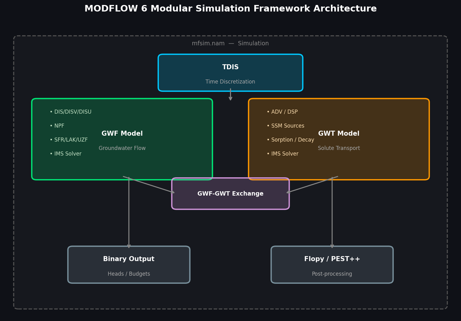
MODFLOW 6 introduces a simulation framework that decouples the numerical engine from individual model definitions. A single simulation can host multiple groundwater flow (GWF) models and groundwater transport (GWT) models that exchange data at every time step through the GWF-GWT exchange and GWF-GWF exchange objects. This design enables:
- Multi-model coupling: adjacent regional and local-scale models share head and flux information without manual boundary interpolation.
- Telescopic mesh refinement: a coarse regional model drives boundary conditions for a fine-scale local model in the same simulation run.
- Simultaneous solute transport: a GWT model reads cell-by-cell flows directly from its paired GWF model, eliminating the file-based coupling that introduced mass-balance errors in older workflows.
The framework is controlled by a plain-text simulation name file (mfsim.nam) that lists all component models, exchanges, and solution groups, making simulation structure transparent and version-controllable.

Unstructured Grids with the DISV and DISU Packages
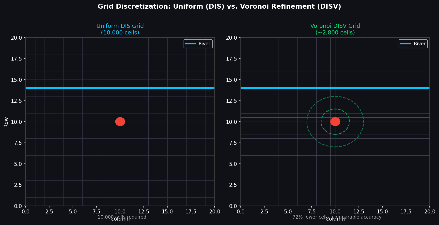
Earlier MODFLOW versions were limited to rectilinear (DIS) grids, forcing modelers to use fine uniform cells in areas of interest—an expensive compromise. MODFLOW 6 adds two unstructured discretization packages:
| Package | Grid Type | Typical Use Case |
|---|---|---|
| DISV | Voronoi / quadtree (vertices shared) | Radial refinement around wells, rivers, or contaminant plumes |
| DISU | Fully unstructured (arbitrary connectivity) | Complex fault zones, karst conduits, or imported geological meshes |
Voronoi grids generated with tools such as Flopy's gridgen module or QGIS plugins allow cell density to increase smoothly near features of interest while keeping total cell counts manageable. Benchmark studies show 3–5× reduction in cell count compared to equivalent uniform grids, with comparable accuracy.
Newton-Raphson Formulation for Unconfined Aquifers
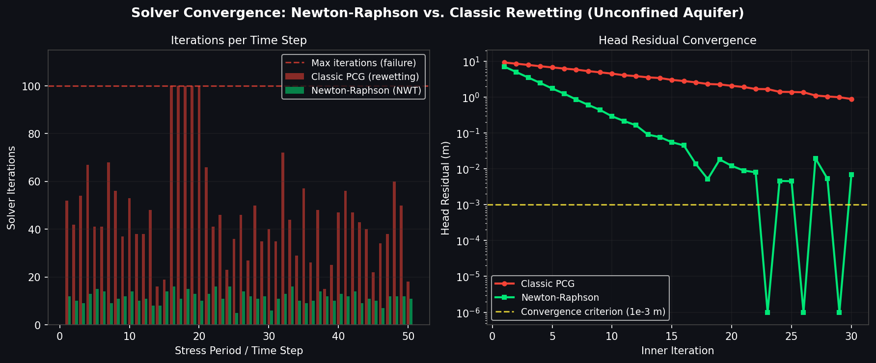
Simulating water-table aquifers with the classic cell-rewetting approach (MODFLOW-2005) is notoriously unstable: cells dry out, rewetting criteria are empirical, and convergence often requires manual iteration. MODFLOW 6 implements a Newton-Raphson (NWT) linearization of the nonlinear unconfined flow equation as the default solver option. Key benefits:
- Cells never truly "dry"—transmissivity smoothly approaches zero as saturated thickness decreases, eliminating rewetting failures.
- Convergence is quadratic near the solution, reducing iteration counts by 40–60% in typical unconfined scenarios.
- The Iterative Model Solution (IMS) package exposes solver parameters (inner/outer iterations, relaxation, preconditioner type) in a single input block, replacing the fragmented PCG/GMG/NWT solver files of earlier versions.
Integrated Surface-Water/Groundwater Interaction
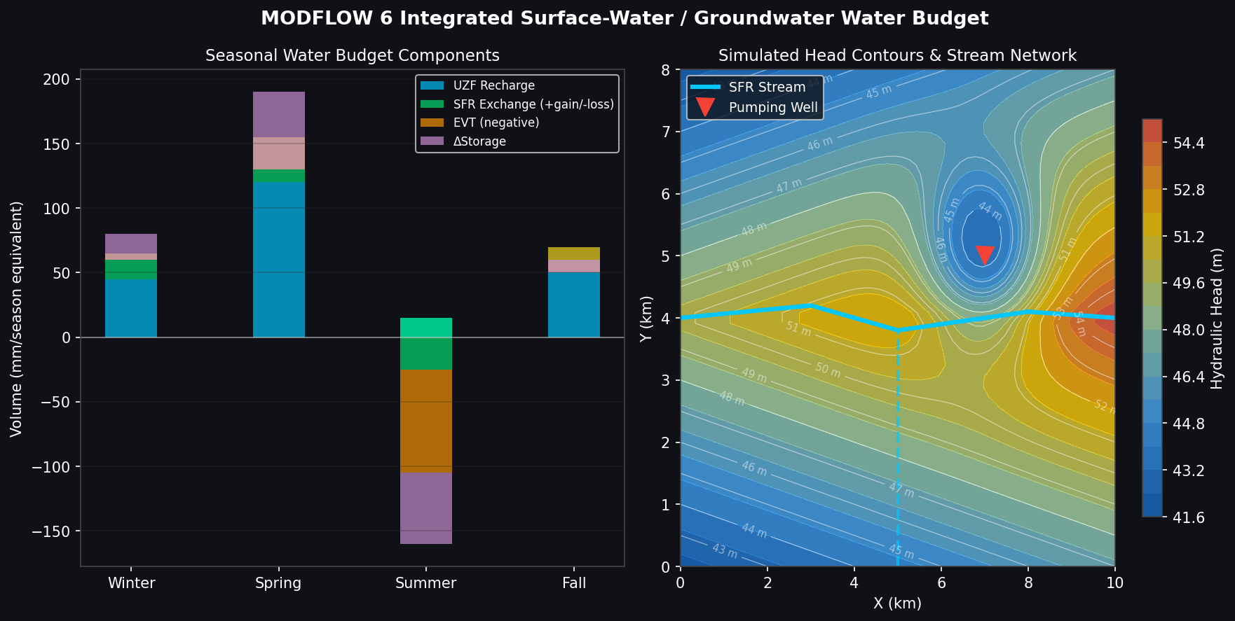
The Streamflow Routing (SFR) package in MODFLOW 6 uses a kinematic-wave approximation to route streamflow through a network of reaches, computing stage-dependent leakage to and from the aquifer at each time step. Combined with the Lake (LAK) and Unsaturated Zone Flow (UZF) packages, a single model can represent:
- Recharge through the vadose zone (UZF)
- Baseflow discharge to streams (SFR)
- Evapotranspiration from shallow water tables (EVT)
- Lake-aquifer exchange with dynamic lake stages (LAK)
This integrated approach is essential for climate-impact studies where changing precipitation patterns alter both recharge rates and streamflow regimes simultaneously.
Solute Transport with the GWT Model
The Groundwater Transport (GWT) model solves the advection-dispersion equation for a single species, supporting:
- Advection schemes: upstream weighting, TVD (third-order), or central-difference
- Dispersion: full 3-D tensor with longitudinal, transverse horizontal, and transverse vertical dispersivities
- Sorption: linear, Freundlich, or Langmuir isotherms
- First-order decay: dual-domain mass transfer for non-equilibrium transport in fractured or heterogeneous media
For multi-species reactive transport, MODFLOW 6 can be coupled externally with PHT3D or RT3D, passing cell-by-cell flows via binary budget files.
Flopy: Python-Based Pre- and Post-Processing
The Flopy library (pip-installable) provides a complete Python API for building, running, and post-processing MODFLOW 6 simulations:
import flopy

sim = flopy.mf6.MFSimulation(sim_name="mymodel", exe_name="mf6")
tdis = flopy.mf6.ModflowTdis(sim, nper=12, perioddata=[(30.0, 10, 1.3)] * 12)
gwf  = flopy.mf6.ModflowGwf(sim, modelname="gwf1", newtonoptions="NEWTON")
dis  = flopy.mf6.ModflowGwfdis(gwf, nlay=3, nrow=100, ncol=100, delr=50.0, delc=50.0)
npf  = flopy.mf6.ModflowGwfnpf(gwf, k=[[10.0], [0.1], [5.0]], icelltype=1)
sim.write_simulation()
sim.run_simulation()
Flopy integrates with matplotlib for head contour maps, pandas for time-series extraction, and xarray for multi-run ensemble analysis—enabling reproducible, script-driven workflows that replace error-prone GUI-based model building.
Practical Workflow: Calibration with PEST++
MODFLOW 6 is fully compatible with PEST++ (Parameter ESTimation), the industry-standard calibration and uncertainty-quantification toolkit. A typical workflow:
- Define pilot points or zones for hydraulic conductivity and storage parameters.
- Run PESTPP-GLM (Gauss-Levenberg-Marquardt) to minimize weighted residuals between simulated and observed heads/flows.
- Use PESTPP-IES (Iterative Ensemble Smoother) for Bayesian parameter estimation with thousands of realizations.
- Propagate parameter uncertainty to forecast quantities (e.g., capture zones, depletion fractions) using PESTPP-SWP.
The combination of MODFLOW 6's binary output, Flopy's post-processing, and PEST++'s ensemble methods enables full uncertainty quantification on groundwater management decisions—a capability that was impractical with earlier MODFLOW versions.
Getting Started
- Download: USGS MODFLOW 6 releases
- Documentation: MODFLOW 6 Input/Output Guide
- Flopy:
pip install flopy— Flopy documentation - PEST++: PEST++ GitHub
- Example notebooks: MODFLOW 6 Examples
MODFLOW 6's modular architecture, unstructured grid support, Newton-Raphson solver, and tight Python integration make it the most capable open-source groundwater modeling platform available. For environmental consultants, water-resource engineers, and hydrogeological researchers, mastering MODFLOW 6 is an investment that pays dividends across the full spectrum of subsurface flow and transport problems.