LISFLOOD-FP: High-Performance Raster-Based 2D Flood Inundation Modeling at Continental Scale

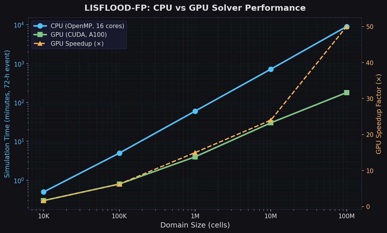
Flood inundation modeling sits at the intersection of hydrology, hydraulics, and risk science. While many tools tackle this problem, LISFLOOD-FP occupies a distinctive niche: a raster-based, storage-cell hydraulic model purpose-built for large-scale, computationally efficient 2D flood simulation. Developed at the University of Bristol and continuously refined over two decades, LISFLOOD-FP has become a reference tool for continental-scale flood hazard mapping, climate impact assessment, and real-time flood forecasting.

What Makes LISFLOOD-FP Different

Most 2D hydraulic solvers—TELEMAC-2D, HEC-RAS 2D, Delft3D—use finite-element or finite-volume schemes on unstructured meshes. These approaches resolve complex flow patterns with high fidelity but scale poorly to catchments spanning thousands of square kilometres. LISFLOOD-FP takes a different path: it discretises the floodplain on a regular raster grid and solves a simplified form of the shallow-water equations (SWE) using an explicit, local inertial approximation.

The local inertial formulation (Bates et al., 2010) retains the pressure and friction terms of the full SWE while dropping the advective acceleration term. This simplification is valid for subcritical, gradually varied flow—the dominant regime in lowland floodplains—and reduces the computational stencil to a single-cell operation, enabling GPU acceleration and massive parallelism.

Solver Options

LISFLOOD-FP ships with four interchangeable solvers:

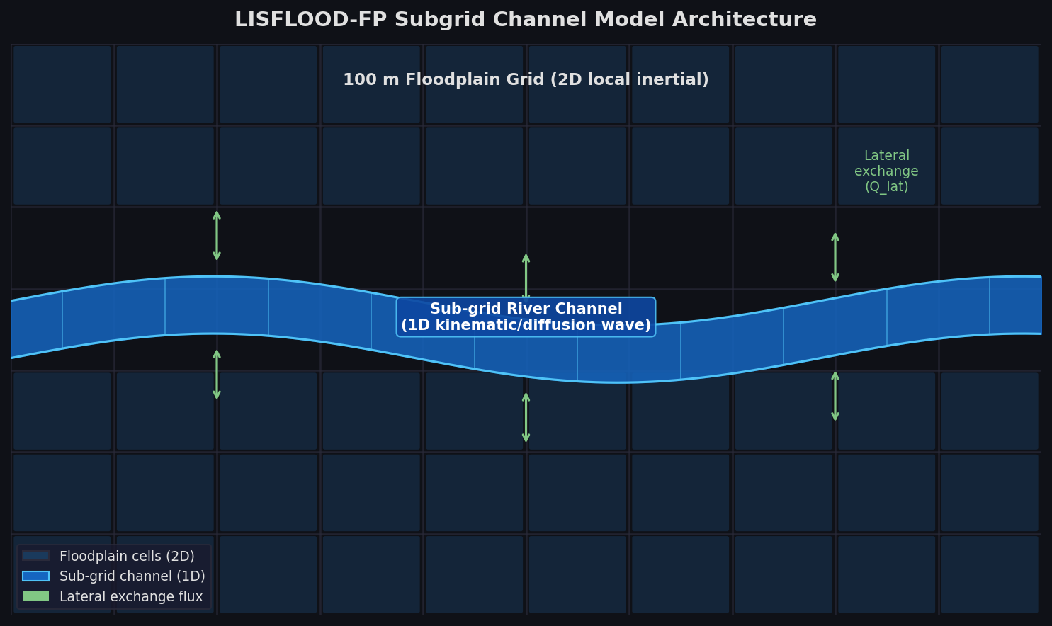
The subgrid channel model (sub) is particularly powerful: it represents the river channel at sub-grid resolution using a 1D kinematic or diffusion-wave approximation, while the floodplain is solved on the coarser raster. This allows a 30 m DEM to drive a 100 m floodplain grid without losing channel geometry detail—a critical capability when working with freely available global DEMs such as MERIT Hydro or FABDEM.

Setting Up a LISFLOOD-FP Simulation

A minimal simulation requires three input files:

1. DEM raster (.dem or GeoTIFF) — the terrain grid defining cell elevations.
2. Parameter file (.par) — controls solver choice, time step, output frequency, and boundary conditions.
3. Boundary condition file (.bci) / boundary condition data (.bdy) — specifies inflow hydrographs, stage boundaries, or rainfall inputs.

A typical .par file excerpt:

DEMfile        catchment.dem
startfile      initial_depth.wd
resroot        output/run01
saveint        3600
massint        300
sim_time       259200
initial_tstep  10
acceleration

The acceleration keyword activates the local inertial solver. Setting gpu instead routes computation to a CUDA-capable GPU, often achieving 50–200× speedup over the CPU solver for large domains.

Boundary Conditions

LISFLOOD-FP supports four boundary condition types:

• QVAR — time-varying discharge hydrograph (most common for river inflows)
• HVAR — time-varying water surface elevation (tidal or downstream stage)
• HFIX — fixed water level (steady-state downstream boundary)
• FREE — free outflow (critical flow at domain edge)

For pluvial flooding, the rainfall module accepts spatially uniform or gridded precipitation (NetCDF), routing excess rainfall directly onto the DEM after subtracting infiltration losses via a Green-Ampt or simple loss-rate model.

GPU Acceleration and Continental-Scale Applications

The GPU solver (lisflood-fp-gpu) is the engine behind several landmark large-scale studies. Neal et al. (2012) demonstrated real-time flood forecasting for the River Severn at 50 m resolution; Sampson et al. (2015) produced the first global 30 m flood hazard map using LISFLOOD-FP on a GPU cluster; Wing et al. (2017) validated the model against FEMA flood maps across the contiguous United States.

For a 1 km² domain at 5 m resolution (40,000 cells), a 72-hour simulation completes in under 30 seconds on a modern GPU. Scaling to a 100,000 km² catchment at 30 m resolution (~111 million cells) typically requires 2–6 hours on a single A100 GPU—a task that would take days on a CPU cluster with a full SWE solver.

Coupling with Hydrological Models

LISFLOOD-FP is routinely coupled with:

• LISFLOOD (JRC) — the European Flood Awareness System (EFAS) uses LISFLOOD for rainfall-runoff and LISFLOOD-FP for inundation routing.
• GloFAS — the Global Flood Awareness System drives LISFLOOD-FP with ECMWF ensemble discharge forecasts.
• VIC / mHM / TOPMODEL — research workflows pipe gridded runoff outputs directly into LISFLOOD-FP boundary conditions.

The coupling interface is straightforward: LISFLOOD-FP reads a .bdy file containing a discharge time series, so any model that can write a hydrograph can drive it.

Calibration and Uncertainty Quantification

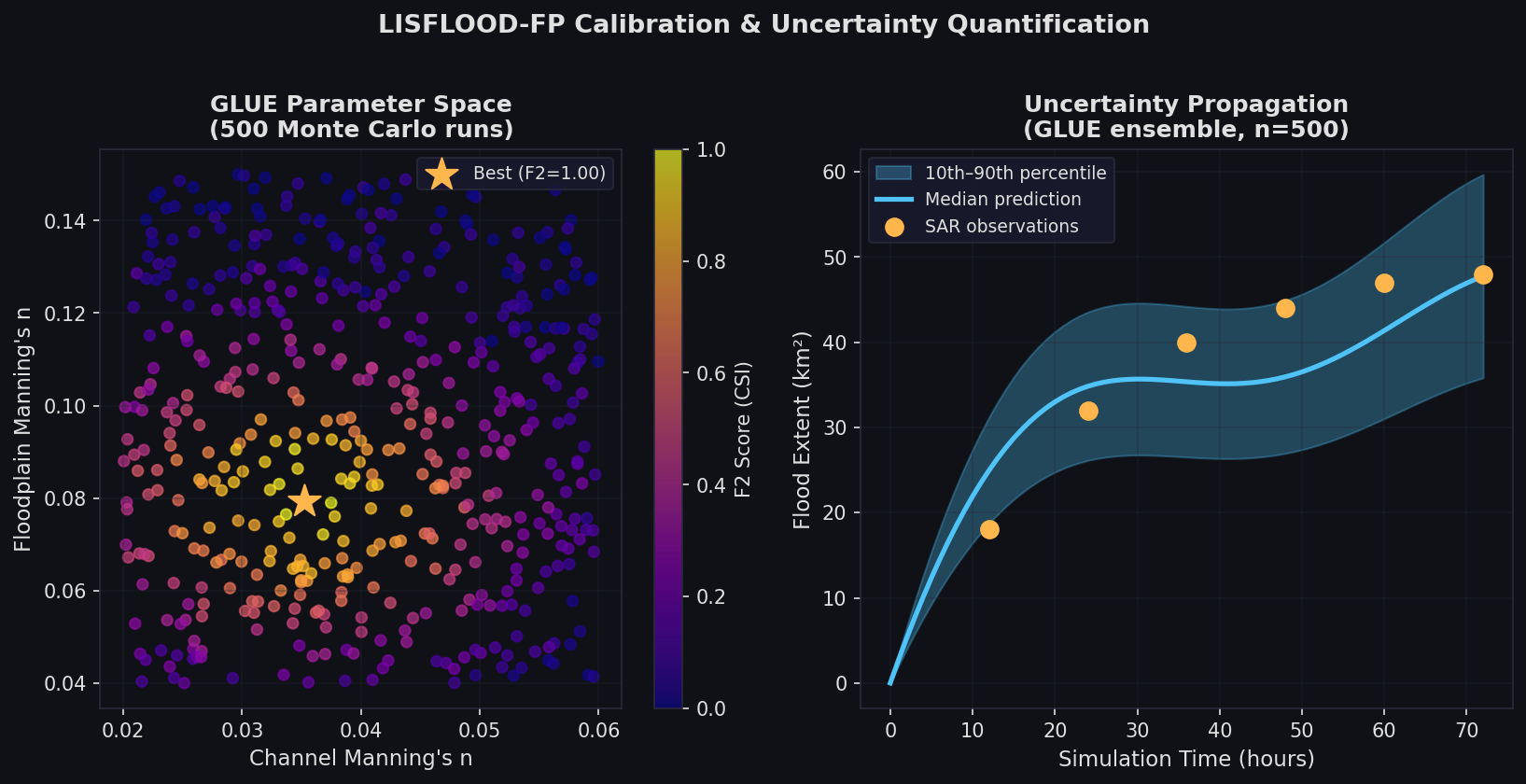
LISFLOOD-FP has two primary calibration parameters: Manning's n for the channel and Manning's n for the floodplain. This parsimony is a deliberate design choice—it makes the model identifiable from sparse observations (flood extent polygons from SAR imagery, peak stage marks) and amenable to Monte Carlo uncertainty analysis.

The standard calibration workflow:

1. Define a prior distribution over channel n (typically 0.02–0.06) and floodplain n (0.04–0.15).
2. Run an ensemble of simulations (100–1,000 parameter sets) using the GLUE (Generalised Likelihood Uncertainty Estimation) framework.
3. Score each run against observed flood extent using the F2 (critical success index) or F (Jaccard) metric derived from SAR-derived inundation maps.
4. Weight parameter sets by likelihood and propagate uncertainty to depth and extent predictions.

Sentinel-1 SAR imagery, freely available via the Copernicus Open Access Hub, has become the standard validation dataset for LISFLOOD-FP calibration at regional to continental scales.

Output Analysis and Visualisation

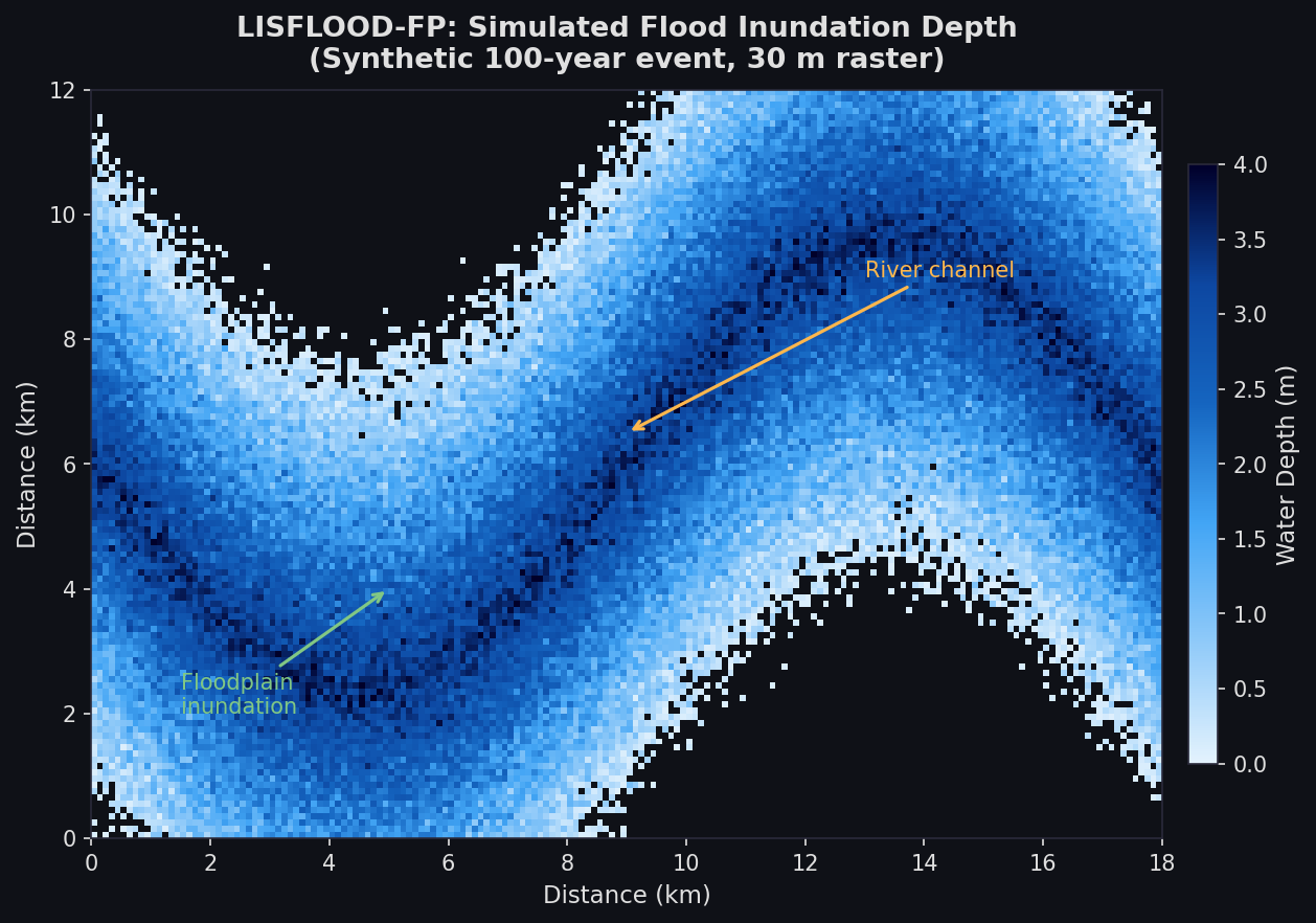
LISFLOOD-FP writes outputs as binary raster files (.wd for water depth, .elev for water surface elevation) at user-specified intervals. Post-processing is typically done in Python:

import numpy as np
import matplotlib.pyplot as plt

# Load water depth raster
depth = np.fromfile('output/run01_0072.wd', dtype=np.float32)
depth = depth.reshape((nrows, ncols))
depth[depth < 0.01] = np.nan  # mask dry cells

fig, ax = plt.subplots(figsize=(12, 8))
im = ax.imshow(depth, cmap='Blues', vmin=0, vmax=5)
plt.colorbar(im, ax=ax, label='Water depth (m)')
ax.set_title('Flood inundation depth — T=72 h')
plt.tight_layout()
plt.savefig('flood_depth_72h.png', dpi=150)

For ensemble outputs, the lisflood-fp-postprocess utilities compute maximum depth envelopes, flood frequency maps, and damage estimates when combined with depth-damage functions.

Practical Considerations

DEM quality is the dominant uncertainty source. LISFLOOD-FP's raster architecture means errors in the DEM propagate directly into flow paths. FABDEM (Forest And Buildings removed Copernicus DEM) consistently outperforms SRTM and raw Copernicus DEM for floodplain applications by removing vegetation and building artefacts.

Time step stability. The explicit solver requires the Courant–Friedrichs–Lewy (CFL) condition: Δt ≤ Δx / √(gH). For a 30 m grid and 5 m depth, this limits Δt to ~4 seconds. The model auto-adjusts the time step, but very deep, fast flows can slow simulations significantly.

Parallelism strategy. For CPU runs, LISFLOOD-FP uses OpenMP shared-memory parallelism. For multi-node HPC, the recommended approach is domain decomposition via MPI wrappers (available in the research branch). GPU runs are single-device; multi-GPU support requires manual domain splitting.

Further Resources

• Source code and documentation: https://www.seamlesswave.com/LISFLOOD8.0
• Original local inertial paper: Bates, P.D., Horritt, M.S., Fewtrell, T.J. (2010). A simple inertial formulation of the shallow water equations for efficient two-dimensional flood inundation modelling. Journal of Hydrology, 387(1–2), 33–45.
• Global flood hazard map: Sampson, C.C. et al. (2015). A high-resolution global flood hazard model. Water Resources Research, 51(9), 7358–7381.
• FABDEM: Hawker, L. et al. (2022). A 30 m global map of elevation with forests and buildings removed. Environmental Research Letters, 17(2), 024016.
• GloFAS integration: https://www.globalfloods.eu
• Copernicus SAR data: https://scihub.copernicus.eu

LISFLOOD-FP's combination of computational efficiency, physical transparency, and proven scalability makes it the tool of choice when flood risk questions span river basins, nations, or continents. Its open-source availability and active research community ensure it will remain at the frontier of large-scale flood inundation science.