FEniCSx for Computational Mechanics of Materials: Finite Element Simulation of Fracture, Plasticity, and Multiphysics Coupling

Continuum-scale materials simulation bridges the gap between atomistic models and engineering components. While molecular dynamics and DFT tools dominate the nanoscale, the FEniCS Project — and its modern successor FEniCSx — provides a powerful, open-source finite element framework for solving the partial differential equations (PDEs) that govern deformation, fracture, heat transfer, and coupled multiphysics phenomena in solid materials.

What Is FEniCSx?

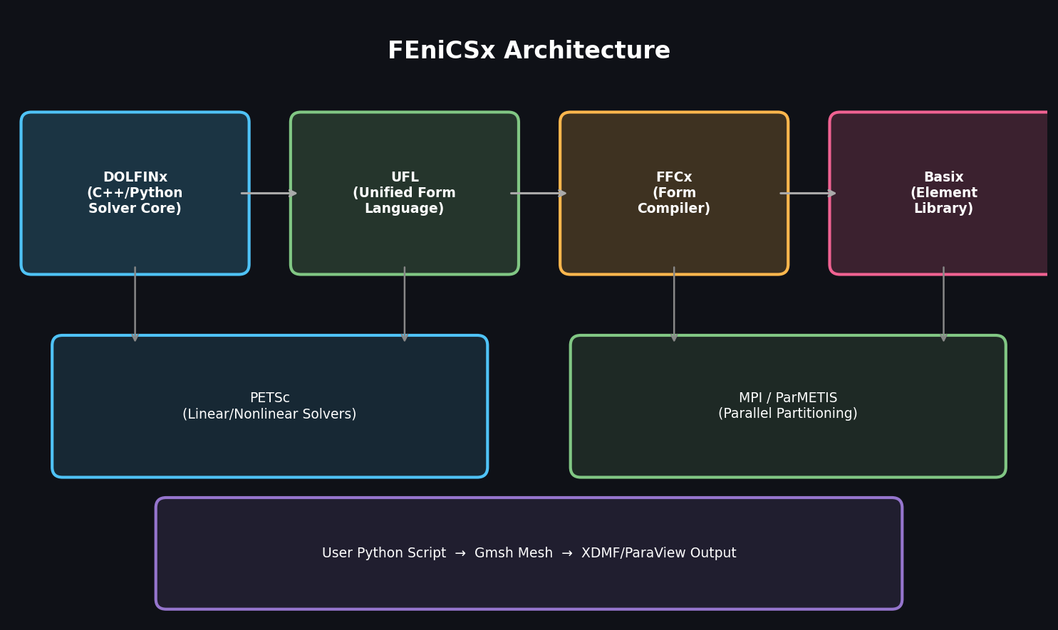
FEniCSx is the next-generation release of the FEniCS computing platform, rewritten from the ground up for performance, flexibility, and Python 3 compatibility. It consists of several tightly integrated components:

• DOLFINx — the core C++/Python problem-solving environment
• UFL (Unified Form Language) — a domain-specific language for expressing variational forms symbolically
• FFCx — the FEniCS Form Compiler that generates optimized C code from UFL expressions
• Basix — a finite element definition library supporting a wide range of element families

Together, these components allow materials scientists and engineers to implement complex constitutive models — from linear elasticity to nonlinear plasticity and phase-field fracture — with concise, readable Python code that compiles to high-performance parallel solvers.

Defining Constitutive Models with UFL

One of FEniCSx's most powerful features is the ability to express material constitutive laws symbolically. For a hyperelastic Neo-Hookean solid, the strain energy density function is written directly in UFL:

from dolfinx import fem, mesh
from ufl import *

# Kinematics
d = len(u)
I = Identity(d)
F = I + grad(u)          # Deformation gradient
C = F.T * F              # Right Cauchy-Green tensor
Ic = tr(C)
J = det(F)

# Neo-Hookean stored energy
mu, lmbda = 80e3, 120e3  # Lamé parameters (Pa)
psi = (mu/2)*(Ic - 3) - mu*ln(J) + (lmbda/2)*(ln(J))**2

# Weak form via automatic differentiation
Pi = psi*dx - dot(B, u)*dx - dot(T, u)*ds
F_form = derivative(Pi, u, v)
J_form = derivative(F_form, u, du)

UFL's automatic differentiation computes the consistent tangent stiffness matrix J_form symbolically — eliminating the error-prone manual derivation of Jacobians that plagues custom FEM codes.

Phase-Field Modeling of Brittle Fracture

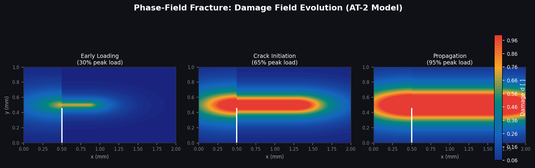
Phase-field fracture has become the method of choice for simulating crack nucleation, propagation, and branching without explicit crack tracking. FEniCSx is particularly well-suited for this approach because the governing equations — a coupled displacement-damage system — map naturally onto its variational framework.

The AT-2 (Ambrosio-Tortorelli) phase-field model introduces a scalar damage field d ∈ [0,1] and minimizes the total energy:

Ψ_total = ∫ [(1-d)² ψ_e(ε) + Gc/(4ℓ)(d² + ℓ²|∇d|²)] dΩ

where Gc is the critical energy release rate and ℓ is the regularization length scale. In FEniCSx, both the elasticity and phase-field equations are solved in a staggered scheme:

1. Elasticity sub-problem: solve for displacement u with fixed damage d
2. Damage sub-problem: solve for d with fixed u, subject to irreversibility constraint d ≥ d_prev

The irreversibility constraint is enforced via a dolfinx.fem.petsc.NonlinearProblem with bound-constrained optimization (SNES VI solver in PETSc), making FEniCSx one of the few open-source platforms that handles this correctly out of the box.

Crystal Plasticity via Custom Quadrature

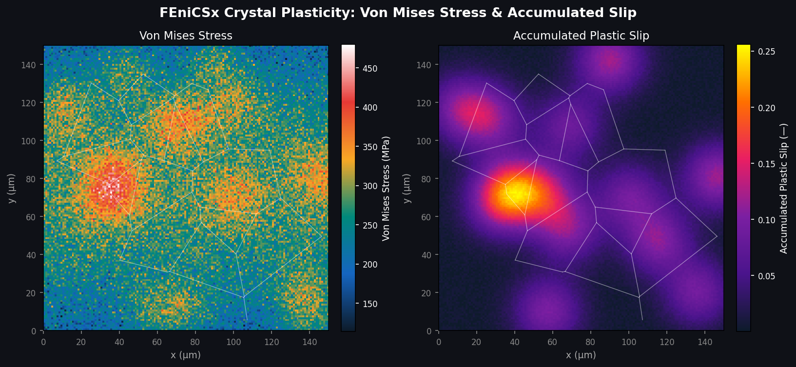
For polycrystalline metals, crystal plasticity finite element (CPFE) models track slip on individual crystallographic systems. FEniCSx supports custom quadrature spaces — storing internal state variables (slip resistance, accumulated plastic strain per slip system) at Gauss points without projecting them onto nodal fields:

from dolfinx.fem import functionspace
from basix.ufl import quadrature_element

# Create quadrature space for 12 FCC slip systems
QE = quadrature_element(domain.topology.cell_name(), 
                         value_shape=(12,), degree=2)
Q = functionspace(domain, QE)
gamma_dot = fem.Function(Q)  # Slip rates per system

This approach avoids the smoothing artifacts that arise when projecting discontinuous internal variables onto continuous nodal fields, preserving the sharp grain-boundary gradients that drive localization.

Multiphysics: Thermo-Mechanical Coupling

Materials processing simulations — welding, additive manufacturing, hot forming — require coupled thermal and mechanical analysis. FEniCSx handles this through operator splitting or monolithic coupling. A typical staggered thermo-mechanical scheme:

1. Solve heat equation with temperature-dependent conductivity and volumetric heat source
2. Update thermal strains: ε_th = α(T)(T - T_ref) I
3. Solve mechanical equilibrium with total strain ε = ε_e + ε_th + ε_p

The same UFL symbolic framework handles both sub-problems, and PETSc's fieldsplit preconditioner enables efficient monolithic solves for tightly coupled systems.

Parallel Scalability and HPC Deployment

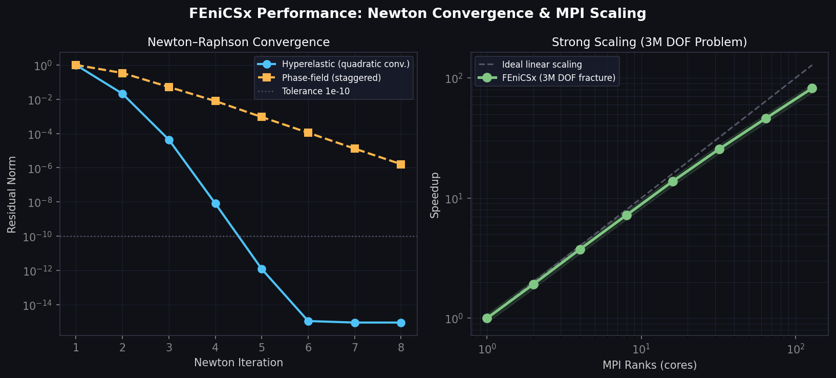
FEniCSx is built on MPI-parallel data structures throughout. Mesh partitioning uses SCOTCH or ParMETIS, and the assembled linear systems are solved with PETSc's suite of parallel direct (MUMPS, SuperLU_dist) and iterative (GAMG, hypre BoomerAMG) solvers. Scaling studies on representative fracture problems show near-linear strong scaling to hundreds of cores, making FEniCSx viable for production-scale component simulations.

Installation on HPC clusters is straightforward via the official Docker/Singularity containers:

singularity pull docker://dolfinx/dolfinx:stable
singularity exec dolfinx_stable.sif python3 my_simulation.py

Practical Workflow for Materials Scientists

A typical FEniCSx materials simulation workflow:

1. Geometry & meshing: generate meshes with Gmsh (Python API), import via dolfinx.io.gmshio
2. Material model: implement constitutive law in UFL; use dolfinx.fem.Expression for history-dependent updates
3. Boundary conditions: apply Dirichlet BCs via dolfinx.fem.dirichletbc; Neumann BCs via surface integrals in the weak form
4. Solver configuration: choose Newton–Raphson with line search for nonlinear problems; configure PETSc SNES options
5. Post-processing: export to XDMF/HDF5 for ParaView visualization; compute derived quantities (J-integral, stress triaxiality) with dolfinx.fem.assemble_scalar

Key Strengths and Limitations

Strengths:

• Symbolic variational formulation reduces implementation errors
• Automatic differentiation for consistent tangent operators
• Native MPI parallelism; scales to HPC clusters
• Active community; extensive tutorial library at jsdokken.com/dolfinx-tutorial

Limitations:

• Steep learning curve for users unfamiliar with variational methods
• No built-in GUI; pre/post-processing requires Gmsh + ParaView
• Legacy FEniCS (2019.1) and FEniCSx APIs are incompatible — migration required for older codes
• Contact mechanics requires third-party libraries (e.g., dolfinx_contact)

Getting Started

FEniCSx is freely available under the LGPL license. The recommended installation path is via conda:

conda create -n fenicsx-env
conda activate fenicsx-env
conda install -c conda-forge fenics-dolfinx mpich pyvista

The official documentation at fenicsproject.org and the community Discourse forum provide extensive resources. For materials-specific applications, the FEniCS in Computational Material Science tutorial collection covers elasticity, plasticity, and phase-field fracture with complete, reproducible examples.

FEniCSx occupies a unique niche in the materials simulation ecosystem: it offers the flexibility of a research code with the robustness of a production solver, making it an essential tool for computational materials scientists working at the continuum scale.