
ASE (Atomic Simulation Environment): Orchestrating Multi-Code Atomistic Workflows in Python
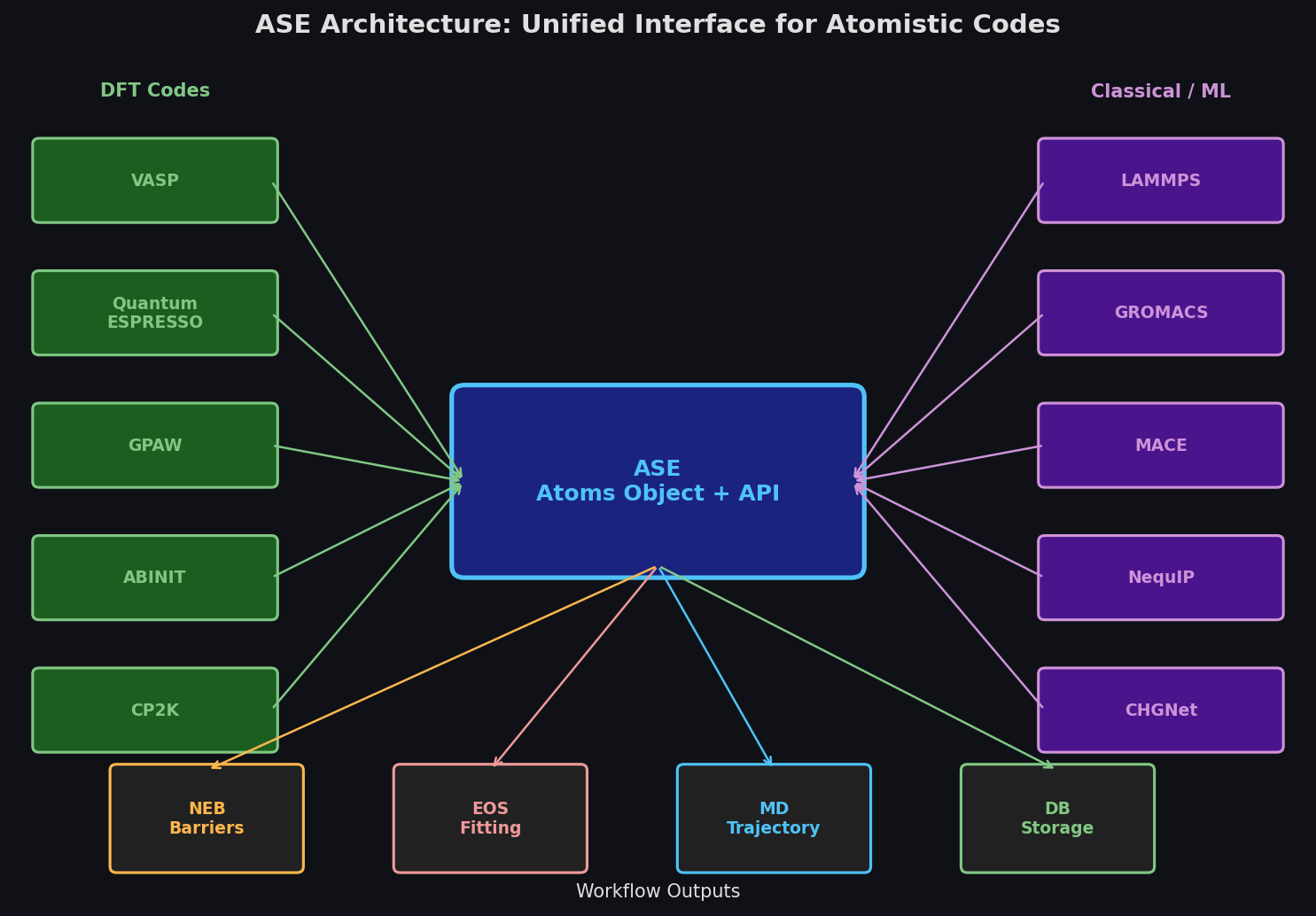
The Atomic Simulation Environment (ASE) has become the connective tissue of modern computational materials science. Rather than being a simulation engine itself, ASE is a Python library that provides a unified interface for setting up, running, and analyzing atomistic calculations across dozens of external codes—from classical force-field engines like LAMMPS to DFT codes such as VASP, Quantum ESPRESSO, and GPAW. For research groups that routinely chain multiple codes together, ASE dramatically reduces the scripting overhead that would otherwise consume weeks of developer time.
What ASE Actually Does
At its core, ASE represents atomic structures as Atoms objects: Python instances that carry atomic positions, species, unit-cell vectors, periodic boundary conditions, and optional arrays for velocities, forces, and charges. Every supported calculator—there are over 30—accepts an Atoms object and returns energies, forces, and stresses in a consistent format. This abstraction means that a geometry-optimization workflow written for VASP can be redirected to Quantum ESPRESSO by changing a single line.
from ase.build import bulk
from ase.calculators.espresso import Espresso
from ase.optimize import BFGS

atoms = bulk('Cu', 'fcc', a=3.61)
atoms.calc = Espresso(pseudopotentials={'Cu': 'Cu.pbe-dn-kjpaw_psl.1.0.0.UPF'},
                      kpts=(8, 8, 8), ecutwfc=60)

opt = BFGS(atoms, trajectory='cu_relax.traj')
opt.run(fmax=0.01)  # eV/Å
print(f"Relaxed lattice constant: {atoms.cell[0,0]:.4f} Å")
The BFGS optimizer, the trajectory writer, and the convergence criterion are all ASE-native; only the Espresso calculator line is code-specific.

Key Capabilities for Materials Workflows
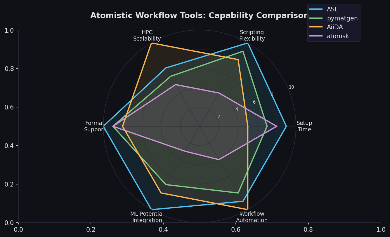
Structure Generation and Manipulation
ASE ships with builders for common crystal structures (bulk, surface, nanotube, molecule), slab generators with configurable vacuum layers, and tools for creating grain boundaries and point defects. The ase.build.make_supercell function accepts an arbitrary transformation matrix, enabling the construction of commensurate supercells for interface modeling or phonon calculations.
For reading and writing structure files, ase.io supports over 40 formats—CIF, POSCAR, XYZ, extXYZ, NetCDF, HDF5, and more—making ASE the de facto format converter in many workflows.
Equation of State and Elastic Constants
The ase.eos module fits Birch-Murnaghan, Vinet, and other equations of state to energy-volume data, extracting bulk modulus and equilibrium volume with a few lines of code. Elastic constant tensors can be computed via finite differences using ase.constraints to apply controlled strains, then fitting the resulting stress tensor components.
Nudged Elastic Band (NEB) for Transition States
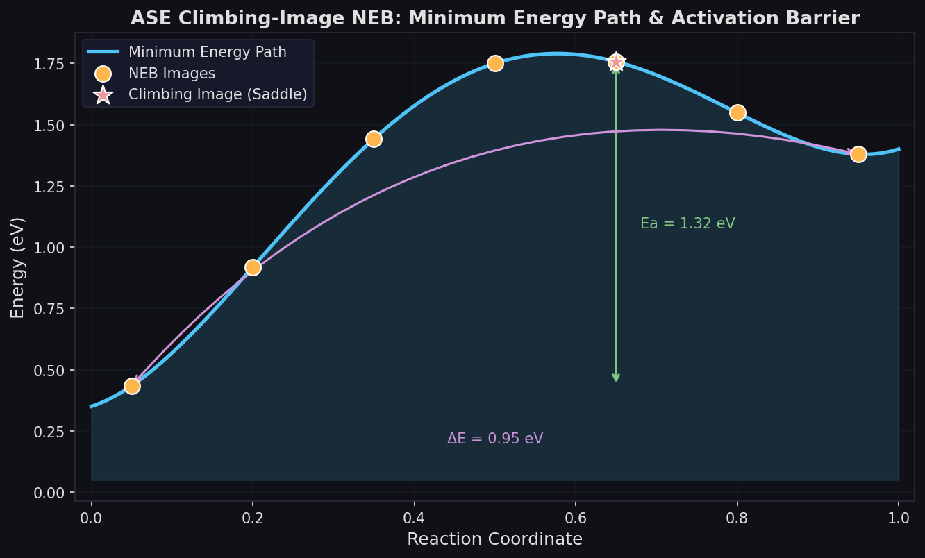
ASE's NEB implementation is one of its most-used features in catalysis and diffusion research. A chain of images between initial and final states is optimized simultaneously, with spring forces keeping images evenly spaced along the minimum-energy path. The climbing-image variant (CI-NEB) drives the highest-energy image to the true saddle point:
from ase.neb import NEB
from ase.optimize import MDMin

images = [initial] + [initial.copy() for _ in range(5)] + [final]
neb = NEB(images, climb=True)
neb.interpolate()

opt = MDMin(neb, trajectory='neb.traj')
opt.run(fmax=0.05)
Activation barriers extracted this way feed directly into kinetic Monte Carlo models or Arrhenius-based rate estimates.
Molecular Dynamics
ASE provides Velocity Verlet, Langevin, and NPT (Nosé-Hoover) integrators. While these are not as performant as dedicated MD engines for million-atom runs, they are ideal for short exploratory trajectories, equilibration protocols, and testing new interatomic potentials before deploying them in LAMMPS or GROMACS.
Machine-Learning Potential Integration
ASE has become the standard interface for machine-learning interatomic potentials (MLIPs). Libraries such as MACE, SchNet, NequIP, and CHGNet all expose ASE-compatible calculators. This means that a potential trained on DFT data can be dropped into any ASE workflow—NEB, MD, geometry optimization—without modification. The ase.calculators.mixing module even supports linear combinations of calculators, useful for QM/MM-style setups.
Database and High-Throughput Workflows
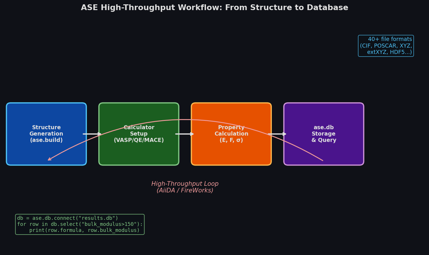
The ase.db module provides a lightweight SQLite or PostgreSQL database for storing and querying Atoms objects alongside computed properties. Each row can carry arbitrary key-value metadata, enabling filtering like:
import ase.db
db = ase.db.connect('results.db')
for row in db.select('bulk_modulus>150, natoms<10'):
    print(row.formula, row.bulk_modulus)
For high-throughput screening, ASE integrates naturally with workflow managers such as AiiDA and FireWorks. AiiDA's ase plugin wraps ASE calculators as AiiDA CalcJob nodes, providing provenance tracking, automatic restart on failure, and remote HPC submission—all while preserving the familiar ASE API.
Practical Considerations
Performance: ASE's Python overhead is negligible compared to DFT wall times, but for classical MD with millions of atoms, use LAMMPS directly. ASE's MD integrators are single-threaded and not suitable for production-scale runs.
Calculator setup: Each calculator requires its own input-file conventions and pseudopotential paths. ASE does not abstract these away—you still need to understand the underlying code's parameters. The ASE calculator documentation lists required and optional keywords for each supported code.
Visualization: ASE's built-in ase.visualize.view launches ASE's own GUI or delegates to VESTA, Avogadro, or Ovito depending on what is installed. For publication-quality renders, export to CIF or POSCAR and use VESTA or OVITO directly.
Getting Started
ASE is available via pip and conda:
pip install ase
# or
conda install -c conda-forge ase
The ASE tutorials cover everything from bulk relaxation to NEB calculations. The ASE GitLab repository hosts the source, issue tracker, and merge-request workflow for contributing new calculators or features.
For groups already using VASP, Quantum ESPRESSO, or LAMMPS, adding ASE to the workflow costs an afternoon of setup and pays dividends in reproducibility, portability, and the ability to swap codes without rewriting analysis scripts. It is the closest thing computational materials science has to a universal adapter.