

Finite Difference Methods for PDE-Based Option Pricing: A Practitioner's Guide
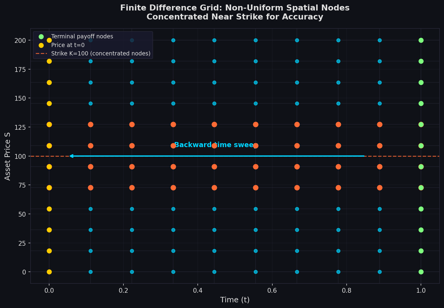
Stochastic volatility models and Monte Carlo engines dominate modern derivatives desks, yet finite difference methods (FDMs) remain the workhorse for pricing vanilla and barrier options when speed and Greeks accuracy are paramount. By discretizing the Black-Scholes PDE—or its extensions—on a structured grid, FDMs deliver deterministic, reproducible prices with analytical-quality sensitivities at a fraction of the computational cost of simulation-based approaches.
Why Finite Differences Over Monte Carlo?
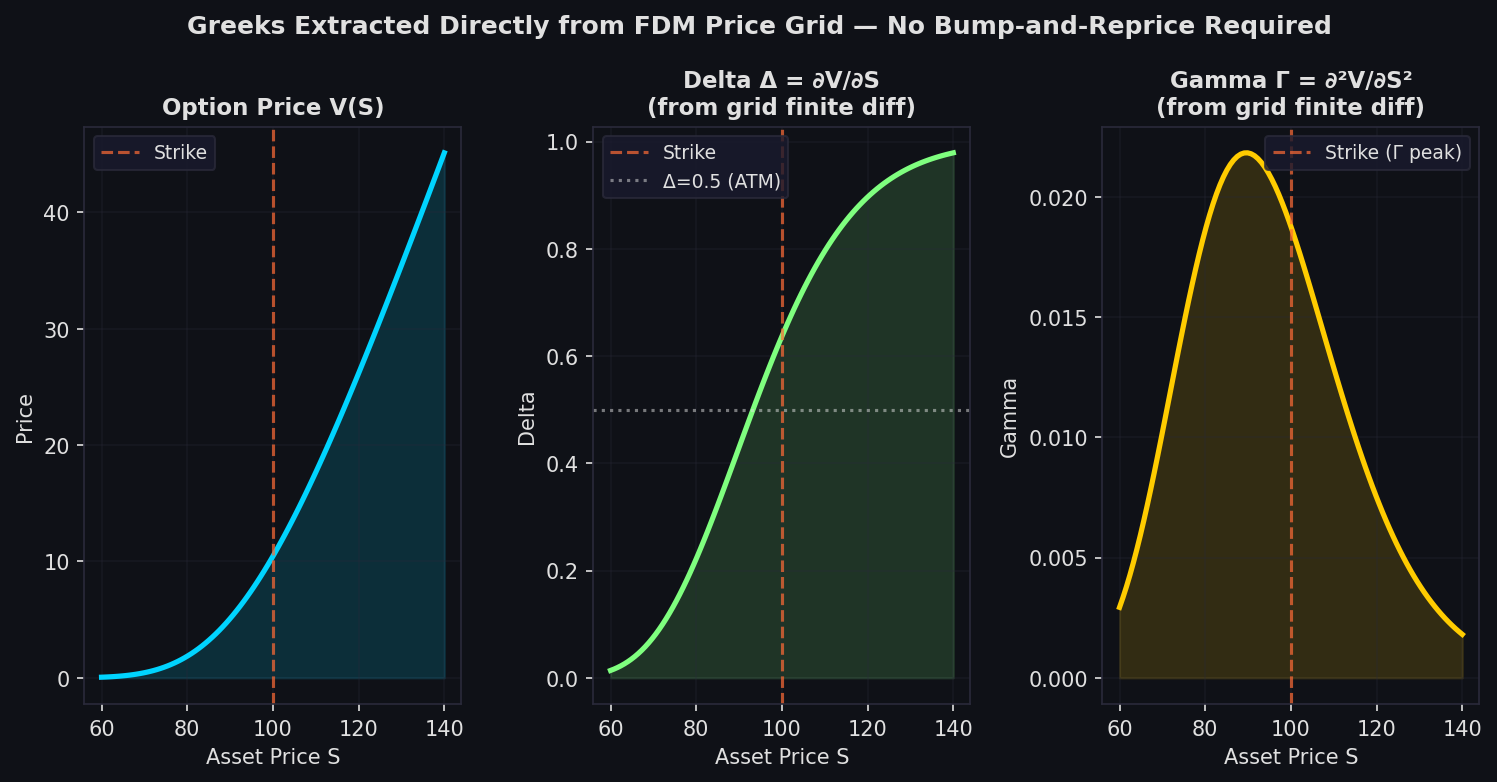
Monte Carlo simulation excels at high-dimensional problems and path-dependent exotics, but it carries inherent statistical noise that complicates delta and gamma hedging. FDMs, by contrast, solve the pricing PDE directly on a grid of asset prices and time steps, producing smooth price surfaces from which Greeks are extracted by simple finite differencing of adjacent grid nodes—no bump-and-reprice required.
For a European call under Black-Scholes, the governing PDE is:

$$\frac{\partial V}{\partial t} + \frac{1}{2}\sigma^2 S^2 \frac{\partial^2 V}{\partial S^2} + rS\frac{\partial V}{\partial S} - rV = 0$$
FDMs replace the continuous derivatives with discrete approximations on a $(S, t)$ grid, marching backward from the known terminal payoff to the present.
The Three Core Schemes
1. Explicit (Forward Euler)
The explicit scheme updates each interior node using only values from the previous time step:
$$V_i^{n} = \alphai V{i-1}^{n+1} + \beta_i V_i^{n+1} + \gammai V{i+1}^{n+1}$$
Pros: Trivially parallelizable; no linear system to solve.
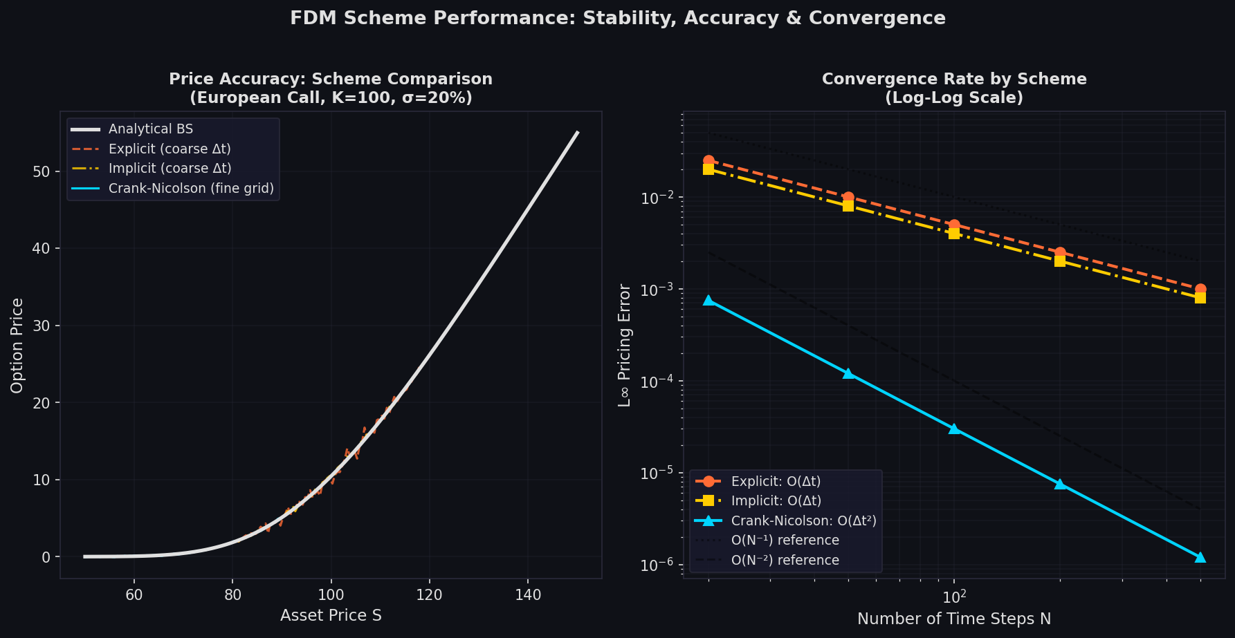
Cons: Conditionally stable—the Courant-Friedrichs-Lewy (CFL) condition forces $\Delta t \leq (\Delta S)^2 / (\sigma^2 S_{\max}^2)$, demanding very fine time steps for reasonable spatial grids.
2. Implicit (Backward Euler)
The implicit scheme couples all nodes at the new time level, requiring a tridiagonal linear solve at each step:
$$-\alphai V{i-1}^{n} + (1 - \beta_i) V_i^{n} - \gammai V{i+1}^{n} = V_i^{n+1}$$
Pros: Unconditionally stable; large time steps are permissible.
Cons: First-order accurate in time ($O(\Delta t)$), introducing temporal diffusion that can smear sharp payoff features.
3. Crank-Nicolson (CN)
CN averages the explicit and implicit operators, achieving second-order accuracy in both space and time ($O(\Delta t^2, \Delta S^2)$):
$$\frac{V_i^n - V_i^{n+1}}{\Delta t} = \frac{1}{2}\mathcal{L}(V^n) + \frac{1}{2}\mathcal{L}(V^{n+1})$$
This is the industry default for vanilla options. However, CN can produce spurious oscillations ("Gibbs phenomenon") near discontinuous payoffs—such as digital options or barrier levels—unless the grid is aligned to the discontinuity or a Rannacher smoothing step (two half-steps of implicit) is applied at initiation.
Grid Construction Best Practices
Non-uniform spatial grids concentrate nodes near the current spot price and the strike, where curvature is highest. A common approach uses a sinh transformation:
$$Sj = S{\max} \cdot \sinh!\left(\frac{j}{N} \cdot \sinh^{-1}!\left(\frac{S_{\max}}{K}\right)\right)$$
This clusters roughly 60–70% of grid points within ±30% of the strike with no increase in total node count.
Time-step control matters near expiry where gamma spikes. Adaptive time stepping—halving $\Delta t$ when the local truncation error exceeds a threshold—maintains accuracy without globally refining the grid.
Boundary conditions must be set carefully:
- At $S = 0$: $V = 0$ for calls; $V = Ke^{-r\tau}$ for puts.
- At $S = S_{\max}$: linear extrapolation (zero gamma) or the asymptotic payoff.
Extending to American Options
American options require enforcing the early-exercise constraint at each time step. The Projected SOR (PSOR) algorithm iterates the tridiagonal solve while projecting each node onto $\max(V_i, \text{intrinsic value})$. Convergence typically requires 5–15 SOR iterations per time step with an optimal relaxation parameter $\omega \approx 1.2$–$1.5$.
Alternatively, the Linear Complementarity Problem (LCP) formulation can be solved directly using the penalty method, which adds a large penalty term to the PDE wherever the option value falls below intrinsic value—avoiding the iterative outer loop entirely.
Greeks from the Grid
One of FDMs' greatest practical advantages is that Greeks emerge naturally from the solved grid:
| Greek | Formula |
|---|---|
| Delta | $(V{i+1} - V{i-1}) / (S{i+1} - S{i-1})$ |
| Gamma | $2(V_{i+1} - 2Vi + V{i-1}) / (S{i+1} - S{i-1})^2$ |
| Theta | $(V_i^{n+1} - V_i^n) / \Delta t$ |
Vega and rho require re-solving the grid with perturbed $\sigma$ or $r$, but the cost is a single additional backward sweep—orders of magnitude cheaper than Monte Carlo re-simulation.
Practical Implementation Considerations
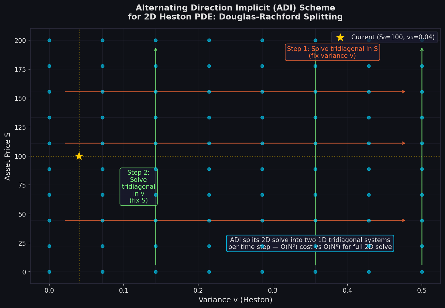
Sparse matrix solvers: For 1D grids (single underlying), Thomas algorithm solves the tridiagonal system in $O(N)$ operations. For 2D grids (e.g., Heston model with stochastic volatility), Alternating Direction Implicit (ADI) schemes—Douglas-Rachford or Craig-Sneyd—split the 2D problem into sequential 1D solves, maintaining tractability.
Calibration integration: FDMs integrate naturally into calibration loops. Because each grid solve is deterministic and fast (milliseconds for a 500×500 grid), iterative Levenberg-Marquardt calibration to market implied volatilities converges reliably without Monte Carlo noise perturbing the objective function.
Parallelization: While a single grid solve is inherently sequential in time, independent strikes, maturities, or scenarios can be solved in parallel across CPU cores or GPU threads. GPU-accelerated FDM libraries (e.g., QuantLib's GPU extensions, custom CUDA kernels) achieve throughput of thousands of option prices per second.
When to Choose FDM
| Scenario | Recommended Method |
|---|---|
| Vanilla European/American options | Crank-Nicolson FDM |
| Barrier options (single barrier) | FDM with grid aligned to barrier |
| Stochastic volatility (Heston) | 2D ADI FDM |
| High-dimensional basket options | Monte Carlo |
| Path-dependent exotics (Asian, lookback) | Monte Carlo or PDE with auxiliary state |
Further Reading
- Wilmott, P., Dewynne, J., & Howison, S. (1993). Option Pricing: Mathematical Models and Computation. Oxford Financial Press.
- Andersen, L. & Piterbarg, V. (2010). Interest Rate Modeling, Vol. 1. Atlantic Financial Press.
- QuantLib FDM Framework Documentation
- Duffy, D. J. (2006). Finite Difference Methods in Financial Engineering. Wiley Finance.
- Haentjens, T. & in 't Hout, K. J. (2012). "Alternating direction implicit finite difference schemes for the Heston–Hull–White PDE." Journal of Computational Finance, 16(1).
Finite difference methods occupy a unique niche in the quantitative finance toolkit: deterministic, fast, and analytically tractable. For any desk pricing vanilla or mildly exotic options under one or two risk factors, a well-implemented FDM grid solver remains the most reliable path from model parameters to hedgeable Greeks.