SABR Model for Interest Rate Derivatives

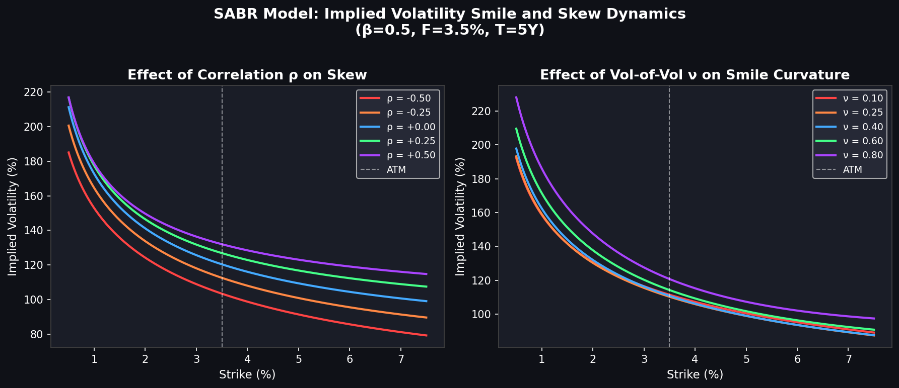
The SABR (Stochastic Alpha Beta Rho) model, introduced by Hagan, Kumar, Lesniewski, and Woodward in their landmark 2002 paper "Managing Smile Risk", has become the dominant framework for modeling implied volatility smiles in interest rate derivatives markets. Unlike the Heston model—which targets equity volatility surfaces—SABR was purpose-built for the interest rate world: caps, floors, swaptions, and CMS products. Its closed-form approximation for implied volatility makes it computationally tractable for real-time calibration, while its stochastic volatility dynamics capture the skew and smile patterns observed in liquid rate markets.

Model Dynamics

SABR models the forward rate $F_t$ and its instantaneous volatility $\sigma_t$ as a coupled system of SDEs under the forward measure:

$$dF_t = \sigma_t F_t^\beta \, dW_t^1$$
$$d\sigma_t = \alpha \sigma_t \, dW_t^2$$
$$dW_t^1 \, dW_t^2 = \rho \, dt$$

The four parameters carry clear financial meaning:

Parameter	Symbol	Interpretation
Initial vol	$\sigma_0$	At-the-money volatility level
Vol-of-vol	$\alpha$	Controls smile curvature
CEV exponent	$\beta$	Controls backbone shape (0=normal, 1=lognormal)
Correlation	$\rho$	Controls skew direction

The $\beta$ parameter is typically fixed by convention: $\beta = 0$ for normal SABR (common in low/negative rate environments), $\beta = 0.5$ for CIR-like dynamics, or $\beta = 1$ for lognormal SABR.

The Hagan Implied Volatility Formula

The key insight of SABR is the closed-form approximation for Black implied volatility $\sigma_{BS}(K, F)$ at strike $K$ and forward $F$:

$$\sigma_{BS}(K, F) \approx \frac{\sigma_0}{(FK)^{(1-\beta)/2} \left[1 + \frac{(1-\beta)^2}{24}\ln^2\frac{F}{K} + \frac{(1-\beta)^4}{1920}\ln^4\frac{F}{K}\right]} \cdot \frac{z}{\chi(z)} \cdot \left[1 + \left(\frac{(1-\beta)^2}{24}\frac{\sigma_0^2}{(FK)^{1-\beta}} + \frac{\rho\beta\alpha\sigma_0}{4(FK)^{(1-\beta)/2}} + \frac{2-3\rho^2}{24}\alpha^2\right)T\right]$$

where $z = \frac{\alpha}{\sigma_0}(FK)^{(1-\beta)/2}\ln\frac{F}{K}$ and $\chi(z) = \ln\frac{\sqrt{1-2\rho z + z^2}+z-\rho}{1-\rho}$.

This formula evaluates in microseconds, making it suitable for real-time Greeks computation and calibration loops over hundreds of strikes.

Calibration to Market Swaption Volatilities

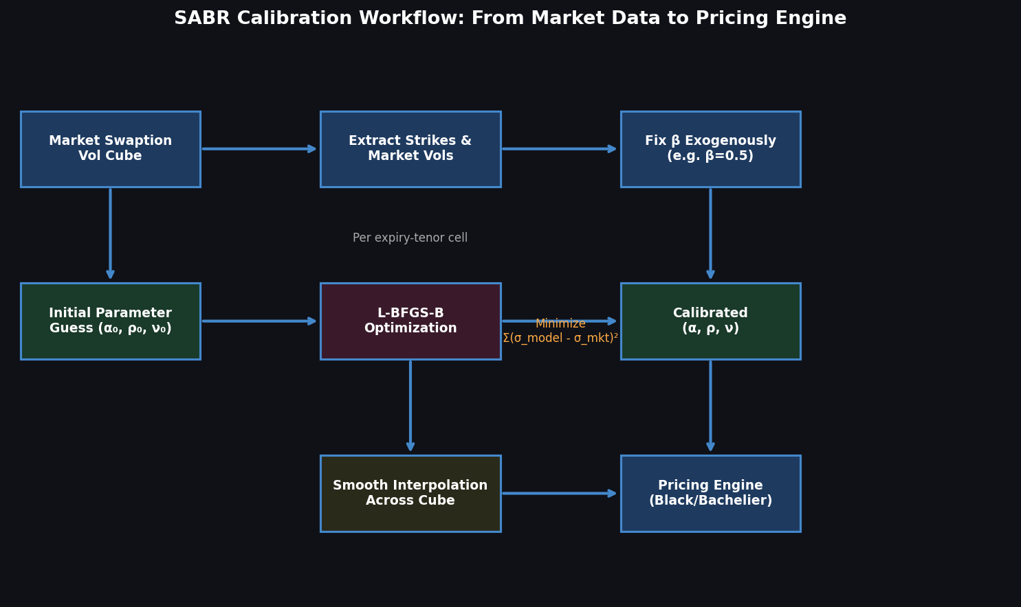
SABR Calibration Workflow from market swaption vol cube to pricing engine

In practice, SABR is calibrated separately for each option expiry and swap tenor (each "expiry-tenor" cell of the swaption cube). The calibration minimizes the sum of squared differences between model and market implied volatilities across strikes:

import numpy as np
from scipy.optimize import minimize
from scipy.stats import norm

def sabr_implied_vol(F, K, T, alpha, beta, rho, nu):
    """Hagan et al. (2002) SABR implied vol approximation."""
    if abs(F - K) < 1e-10:  # ATM formula
        FK_mid = F
        term1 = alpha / (FK_mid ** (1 - beta))
        term2 = 1 + ((1-beta)**2/24 * alpha**2 / FK_mid**(2*(1-beta))
                     + rho*beta*nu*alpha / (4*FK_mid**((1-beta)))
                     + (2 - 3*rho**2)/24 * nu**2) * T
        return term1 * term2

    log_FK = np.log(F / K)
    FK_beta = (F * K) ** ((1 - beta) / 2)

    z = nu / alpha * FK_beta * log_FK
    chi_z = np.log((np.sqrt(1 - 2*rho*z + z**2) + z - rho) / (1 - rho))

    numer = alpha
    denom = FK_beta * (1 + (1-beta)**2/24 * log_FK**2
                       + (1-beta)**4/1920 * log_FK**4)

    correction = 1 + ((1-beta)**2/24 * alpha**2 / FK_beta**2
                      + rho*beta*nu*alpha / (4*FK_beta)
                      + (2 - 3*rho**2)/24 * nu**2) * T

    return numer / denom * (z / chi_z) * correction

def calibrate_sabr(F, T, strikes, market_vols, beta=0.5):
    """Calibrate alpha, rho, nu to market implied vols with fixed beta."""
    def objective(params):
        alpha, rho, nu = params
        if alpha <= 0 or nu <= 0 or abs(rho) >= 1:
            return 1e10
        model_vols = [sabr_implied_vol(F, K, T, alpha, beta, rho, nu)
                      for K in strikes]
        return np.sum((np.array(model_vols) - np.array(market_vols))**2)

    # Initial guess: ATM vol, zero skew, moderate vol-of-vol
    atm_vol = np.interp(F, strikes, market_vols)
    x0 = [atm_vol * F**(1-beta), 0.0, 0.3]
    bounds = [(1e-6, None), (-0.999, 0.999), (1e-6, None)]
    result = minimize(objective, x0, method='L-BFGS-B', bounds=bounds)
    return result.x  # alpha, rho, nu

A typical calibration over 10 strikes completes in under 50 milliseconds, enabling real-time recalibration as market quotes update.

Handling Negative Rates: Shifted SABR

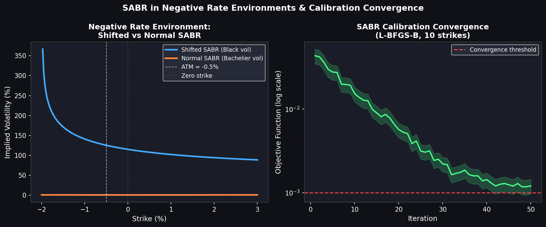
Post-2014, EUR and CHF rates turned negative, breaking the standard lognormal SABR ($\beta=1$) which requires $F > 0$. The industry response was Shifted SABR: apply a shift $s$ so that $F' = F + s$ and $K' = K + s$ remain positive. Common shifts are 1–3% for EUR rates.

def shifted_sabr_vol(F, K, T, alpha, beta, rho, nu, shift=0.02):
    """SABR with additive shift for negative rate environments."""
    return sabr_implied_vol(F + shift, K + shift, T, alpha, beta, rho, nu)

Alternatively, Normal SABR ($\beta=0$) directly models rates as arithmetic Brownian motion, producing Bachelier (normal) implied volatilities that are well-defined for negative rates without any shift.

Integration with QuantLib

SABR in Negative Rate Environments: Shifted vs Normal SABR and calibration convergence

QuantLib provides production-grade SABR calibration via SabrSmileSection and the SabrInterpolatedSmileSection class:

import QuantLib as ql

# Define swaption market data
expiry = ql.Period(5, ql.Years)
tenor  = ql.Period(10, ql.Years)
atm_forward = 0.035  # 3.5% ATM forward swap rate

strikes = [0.01, 0.02, 0.03, 0.035, 0.04, 0.05, 0.06]
vols    = [0.42, 0.35, 0.29, 0.27,  0.26, 0.25, 0.26]  # market normal vols

# Calibrate SABR
sabr_section = ql.SabrSmileSection(
    5.0,           # time to expiry
    atm_forward,
    [0.20, 0.5, -0.30, 0.40],  # initial [alpha, beta, rho, nu]
    ql.SabrApproximation
)

QuantLib's SABR implementation handles the ATM singularity, enforces parameter bounds, and supports multiple approximation variants including the Obloj correction for improved accuracy at long expiries.

Practical Calibration Considerations

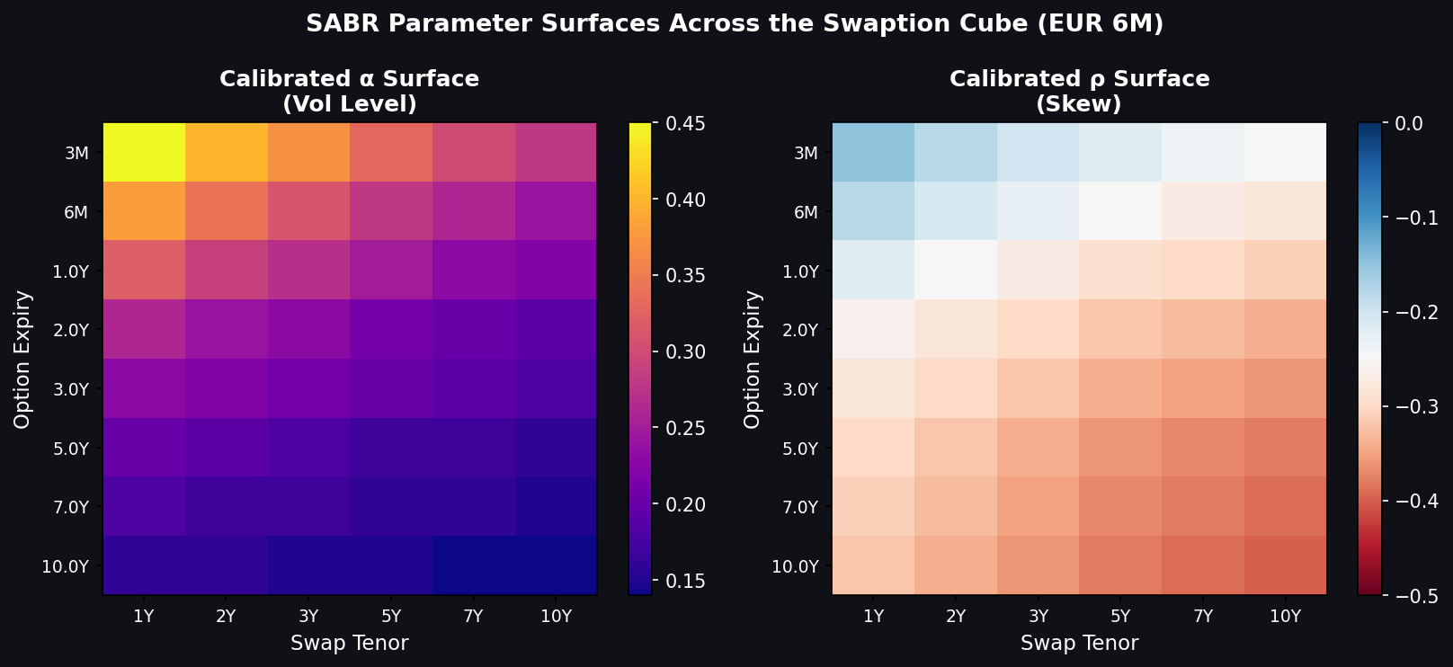
Calibrated SABR Parameter Surfaces (alpha and rho) across the EUR swaption cube

Fixing $\beta$: Most desks fix $\beta$ exogenously (e.g., $\beta=0.5$ for rates) rather than calibrating it, since $\alpha$ and $\beta$ are nearly co-linear in the ATM region. The choice of $\beta$ affects the backbone—how ATM vol moves as the forward moves—which should be validated against historical data.

Regularization: With sparse strike grids (3–5 strikes), the calibration is underdetermined. Adding Tikhonov regularization on $\alpha$ and $\nu$ prevents overfitting and produces smoother parameter surfaces across the swaption cube.

Arbitrage-Free SABR: The Hagan approximation can produce negative probability densities at extreme strikes for long expiries. The Antonov-Konikov-Spector (2013) density-based SABR and Hagan's 2014 PDE-based extension eliminate these arbitrage violations for production use.

Interpolation Across the Cube: After calibrating SABR parameters for each expiry-tenor cell, practitioners interpolate $(\alpha, \rho, \nu)$ surfaces smoothly across the cube using cubic splines or parametric forms, ensuring consistent pricing across all instruments.

Pricing Caps, Floors, and Swaptions

Once calibrated, SABR-implied vols feed directly into Black or Bachelier pricing formulas:

def black_caplet(F, K, T, sigma, notional, tau, is_cap=True):
    """Black formula for a single caplet/floorlet."""
    d1 = (np.log(F/K) + 0.5*sigma**2*T) / (sigma*np.sqrt(T))
    d2 = d1 - sigma*np.sqrt(T)
    if is_cap:
        return notional * tau * (F*norm.cdf(d1) - K*norm.cdf(d2))
    else:
        return notional * tau * (K*norm.cdf(-d2) - F*norm.cdf(-d1))

# Price a cap strip using SABR vols
cap_price = sum(
    black_caplet(F=fwd[i], K=strike, T=expiries[i],
                 sigma=sabr_implied_vol(fwd[i], strike, expiries[i],
                                        *sabr_params[i]),
                 notional=1e6, tau=0.25)
    for i in range(len(expiries))
)

Implementing the SABR Stochastic Volatility Model for Interest Rate Derivatives