Regime-Switching Models for Macroeconomic Stress Testing

Financial markets do not behave uniformly over time. Bull markets, bear markets, high-volatility crises, and low-volatility expansions each exhibit distinct statistical properties. Regime-switching models—most notably the Hamilton Markov-Switching Model—provide a rigorous framework for capturing these structural breaks, making them indispensable for macroeconomic stress testing and scenario analysis.

What Are Regime-Switching Models?

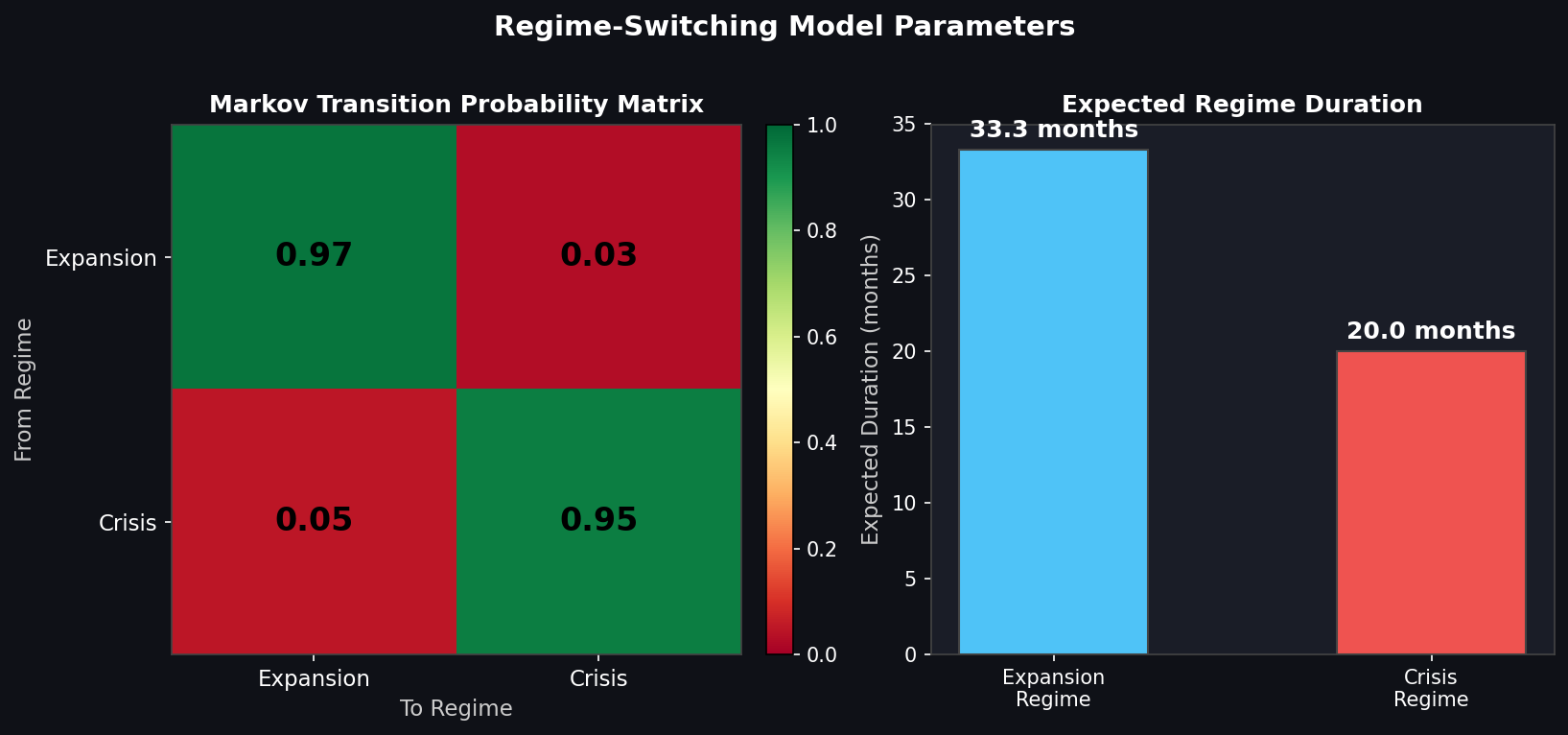
A regime-switching model assumes that the data-generating process transitions between a finite number of latent states (regimes). In a two-regime specification, for example, the economy might alternate between an expansion regime (low volatility, positive drift) and a contraction regime (high volatility, negative drift). The transition between regimes is governed by a Markov chain with a constant transition probability matrix P:

P = | p₁₁  p₁₂ |
    | p₂₁  p₂₂ |

where p_ij is the probability of moving from regime i to regime j in the next period. Each regime has its own mean (μ) and variance (σ²), estimated jointly via the Expectation-Maximization (EM) algorithm or maximum likelihood estimation (MLE).

Why Regime-Switching Models Excel at Stress Testing

Traditional stress tests often rely on historical scenarios or simple shock overlays applied to a single-regime model. This approach underestimates tail risk because it ignores the fact that correlations, volatilities, and return distributions change dramatically across regimes. Regime-switching models address this by:

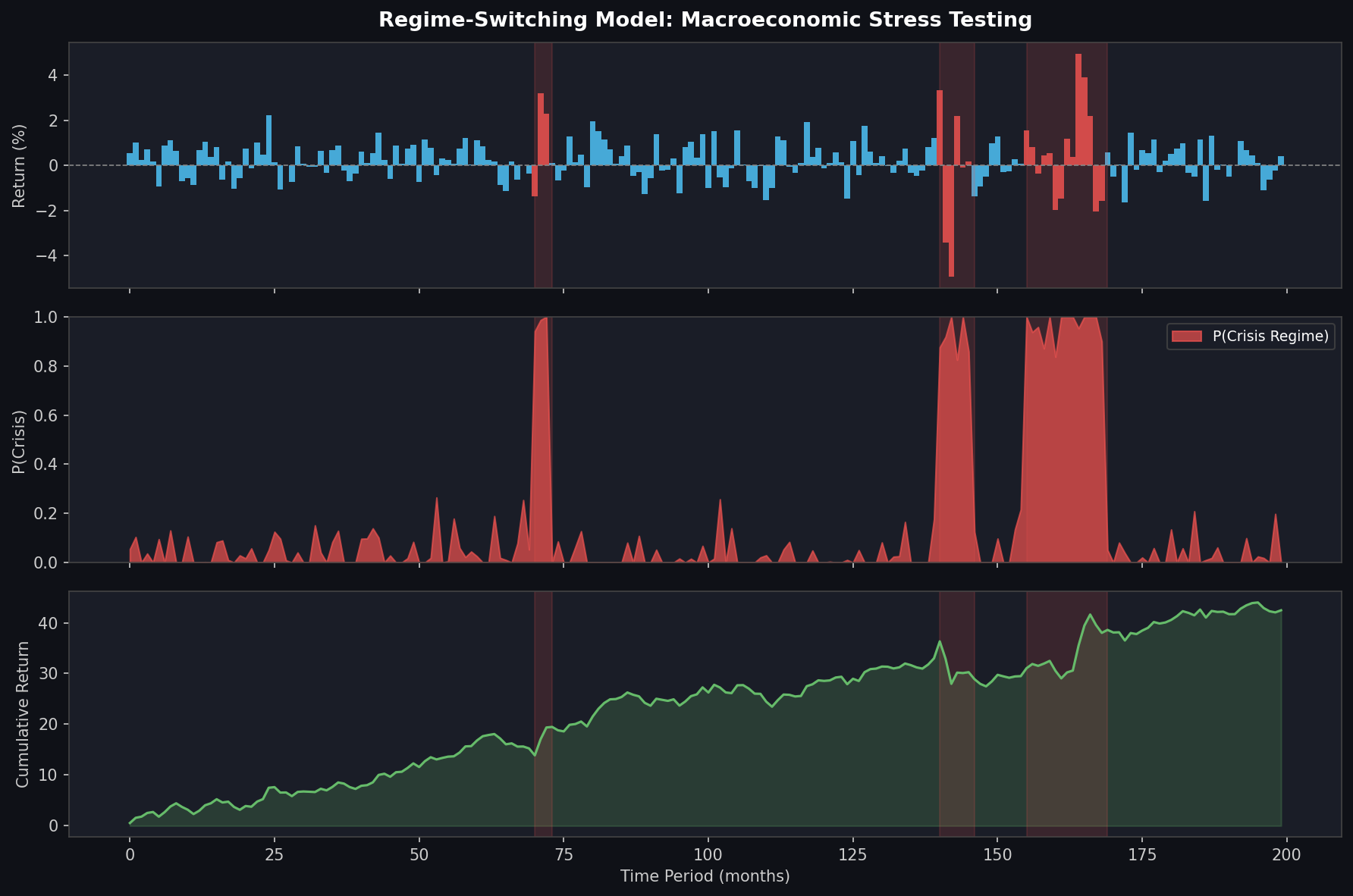
Endogenously identifying crisis periods — The model infers regime probabilities from the data itself, without requiring the analyst to pre-specify crisis dates.
Capturing volatility clustering — Unlike GARCH models (which model conditional heteroskedasticity within a single regime), regime-switching models allow for abrupt, persistent shifts in the volatility level.
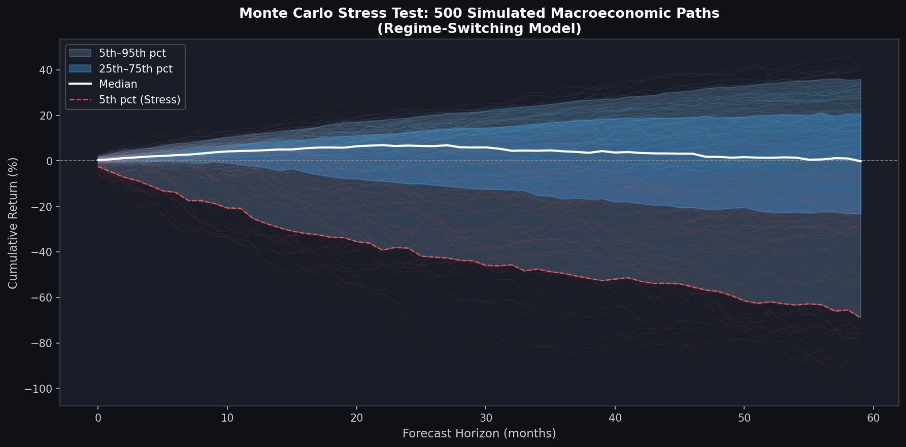
Generating realistic multi-period scenarios — By simulating forward through the Markov chain, analysts can generate thousands of plausible macroeconomic paths, each consistent with historically observed regime dynamics.
Stress-testing correlation structures — In a multi-asset setting, each regime can have its own covariance matrix, capturing the well-documented phenomenon of correlation breakdown during crises.

Practical Implementation in Python

The statsmodels library provides a production-ready implementation of Hamilton's Markov-switching autoregression:

import pandas as pd
import numpy as np
import statsmodels.api as sm

# Load GDP growth or equity return series
returns = pd.read_csv('macro_returns.csv', index_col=0, parse_dates=True)['return']

# Fit a 2-regime Markov-switching model with AR(1) dynamics
mod = sm.tsa.MarkovAutoregression(
    returns,
    k_regimes=2,
    order=1,
    switching_ar=False,       # AR coefficient constant across regimes
    switching_variance=True   # Variance switches across regimes
)
res = mod.fit(search_reps=20, search_iter=100)
print(res.summary())

# Extract smoothed regime probabilities
smoothed_probs = res.smoothed_marginal_probabilities

The smoothed_marginal_probabilities output gives the posterior probability of being in each regime at each time step—a powerful diagnostic for identifying historical crisis periods.

Simulating Forward Paths for Stress Testing

Once the model is calibrated, forward simulation is straightforward:

def simulate_regime_paths(res, n_periods=60, n_simulations=10_000):
    """Simulate n_simulations paths of length n_periods."""
    trans_matrix = res.regime_transition  # Shape: (k_regimes, k_regimes)
    params = res.params
    paths = np.zeros((n_simulations, n_periods))
    regimes = np.zeros((n_simulations, n_periods), dtype=int)

    # Initialize from the ergodic (stationary) distribution
    ergodic = np.linalg.solve(
        (trans_matrix.T - np.eye(2)).T[:-1],
        np.zeros(1)
    )
    # Simplified: start in regime 0 or 1 based on last smoothed probability
    current_regime = np.random.choice(2, size=n_simulations,
                                       p=smoothed_probs.iloc[-1].values)

    for t in range(n_periods):
        regimes[:, t] = current_regime
        mu = np.where(current_regime == 0, params['const[0]'], params['const[1]'])
        sigma = np.where(current_regime == 0,
                         np.sqrt(params['sigma2[0]']),
                         np.sqrt(params['sigma2[1]']))
        paths[:, t] = mu + sigma * np.random.randn(n_simulations)
        # Transition to next regime
        rand = np.random.rand(n_simulations)
        p_stay = trans_matrix[current_regime, current_regime]
        current_regime = np.where(rand < p_stay, current_regime, 1 - current_regime)

    return paths, regimes

paths, regimes = simulate_regime_paths(res)

This produces a distribution of 5-year macroeconomic paths that can be fed directly into portfolio valuation models, credit risk engines, or regulatory capital calculators.

Markov Transition Probability Matrix and Expected Regime Durations

Key Calibration Considerations

Number of regimes: Two regimes (expansion/contraction) suffice for most applications. Three regimes (expansion, moderate stress, severe crisis) improve fit for equity markets but increase estimation complexity.
Data frequency: Monthly or quarterly macroeconomic data is preferred. Daily financial data may require additional filtering to avoid spurious regime switches.
Stationarity: Ensure the input series is stationary (differenced GDP, log-returns) before fitting. Non-stationary inputs lead to degenerate regime estimates.
Regime persistence: Check that estimated transition probabilities imply economically plausible regime durations. A crisis regime lasting on average 2 months is more credible than one lasting 2 weeks.

Monte Carlo Stress Test: 500 Simulated Macroeconomic Paths

Integration with Regulatory Stress Testing Frameworks

Regime-switching models align naturally with regulatory requirements under DFAST (Dodd-Frank Act Stress Testing) and CCAR (Comprehensive Capital Analysis and Review). Regulators require banks to evaluate performance under adverse and severely adverse scenarios. A regime-switching model can:

Quantify the probability of entering a severe-stress regime over a 9-quarter horizon.
Generate internally consistent multi-variable stress scenarios (GDP, unemployment, interest rates) by fitting a Vector Markov-Switching (VMS) model.
Provide a transparent, auditable methodology that satisfies model risk management (MRM) requirements under SR 11-7.

Implementing Regime-Switching Models for Macroeconomic Stress Testing