Kalman Filtering for Dynamic Asset Allocation

In quantitative finance, dynamic asset allocation requires continuous updating of portfolio weights as new market information arrives. Traditional static optimization approaches fail to capture the time-varying nature of expected returns, volatilities, and correlations. Kalman filtering provides a powerful framework for real-time parameter estimation and state tracking in financial models, enabling adaptive portfolio strategies that respond systematically to changing market conditions.

The State-Space Framework for Financial Modeling

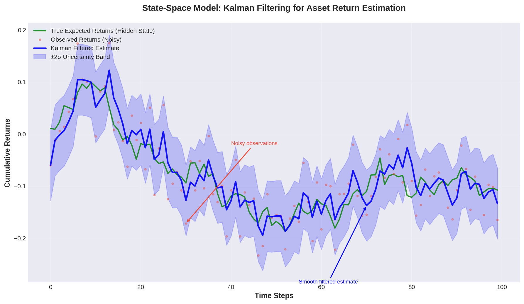
Kalman filtering operates on a state-space representation where unobservable states (such as true expected returns or latent risk factors) evolve according to a linear dynamic system, while observable market data provides noisy measurements of these states. For asset allocation, we typically model expected returns as a hidden state that follows a random walk or mean-reverting process:

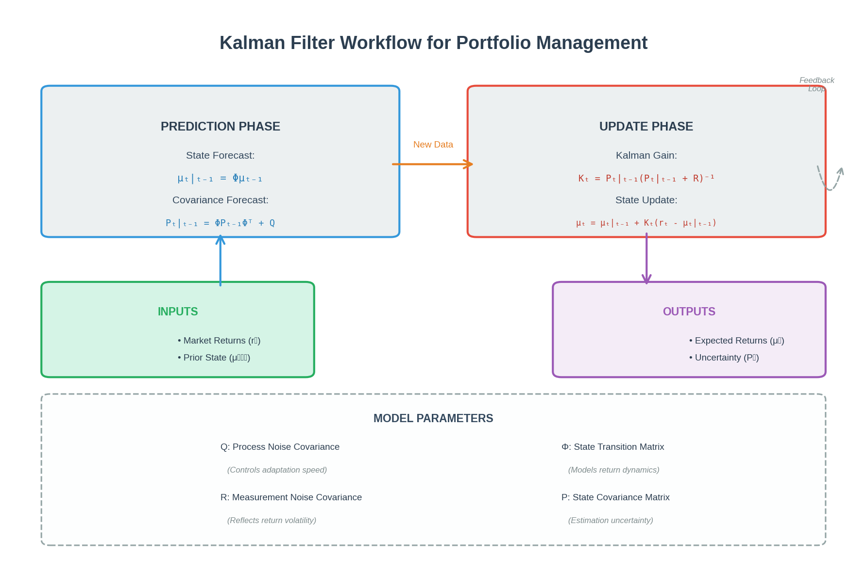
State equation: μₜ = Φμₜ₋₁ + wₜ
Observation equation: rₜ = μₜ + vₜ

Here, μₜ represents the true expected return vector at time t, rₜ is the observed return, Φ is the state transition matrix, and wₜ and vₜ are process and measurement noise terms. The Kalman filter recursively estimates μₜ by optimally combining prior beliefs with new observations, weighted by their respective uncertainties.

Implementation Strategy for Portfolio Applications

State-space model visualization showing hidden states and observed returns

A practical implementation begins with parameter initialization. The state covariance matrix Q (process noise) controls how quickly the filter adapts to regime changes, while the measurement covariance R (observation noise) reflects the volatility of asset returns. These parameters can be estimated from historical data using maximum likelihood or set based on domain knowledge about market dynamics.

The filter operates in two phases: prediction and update. During prediction, we forecast the next state and its uncertainty based on the transition model. When new return data arrives, the update step computes the Kalman gain—a matrix that determines how much to adjust our state estimate based on the prediction error. High Kalman gain indicates we trust the new observation more than our prior estimate.

For multi-asset portfolios, the filter can track a vector of expected returns simultaneously, capturing cross-asset dependencies through the state covariance structure. This enables the model to learn that when one asset's expected return shifts, related assets likely experience similar changes.

Advanced Extensions and Practical Considerations

Real-world financial data often violates the Kalman filter's linearity and Gaussian assumptions. The Extended Kalman Filter (EKF) handles nonlinear state transitions through local linearization, useful when modeling phenomena like stochastic volatility or regime-dependent dynamics. The Unscented Kalman Filter (UKF) offers better performance for highly nonlinear systems by propagating carefully chosen sample points through the nonlinear transformation.

Time-varying parameters present another challenge. Adaptive filtering techniques allow Q and R to evolve over time, automatically adjusting the filter's responsiveness to match current market conditions. During high-volatility periods, increasing Q enables faster adaptation to rapid changes in expected returns.

Integration with portfolio optimization requires careful handling of estimation uncertainty. Rather than treating filtered estimates as known parameters, robust optimization approaches can incorporate the state covariance matrix to account for estimation risk. This prevents over-confident allocation decisions based on noisy parameter estimates.

Performance Monitoring and Validation

Portfolio adaptation comparison between Kalman filtering and static allocation

Effective implementation requires continuous validation of filter performance. Innovation sequences (prediction errors) should exhibit white noise properties if the model is well-specified. Persistent patterns in innovations indicate model misspecification—perhaps the state transition model is too simple, or the noise covariances are incorrectly specified.

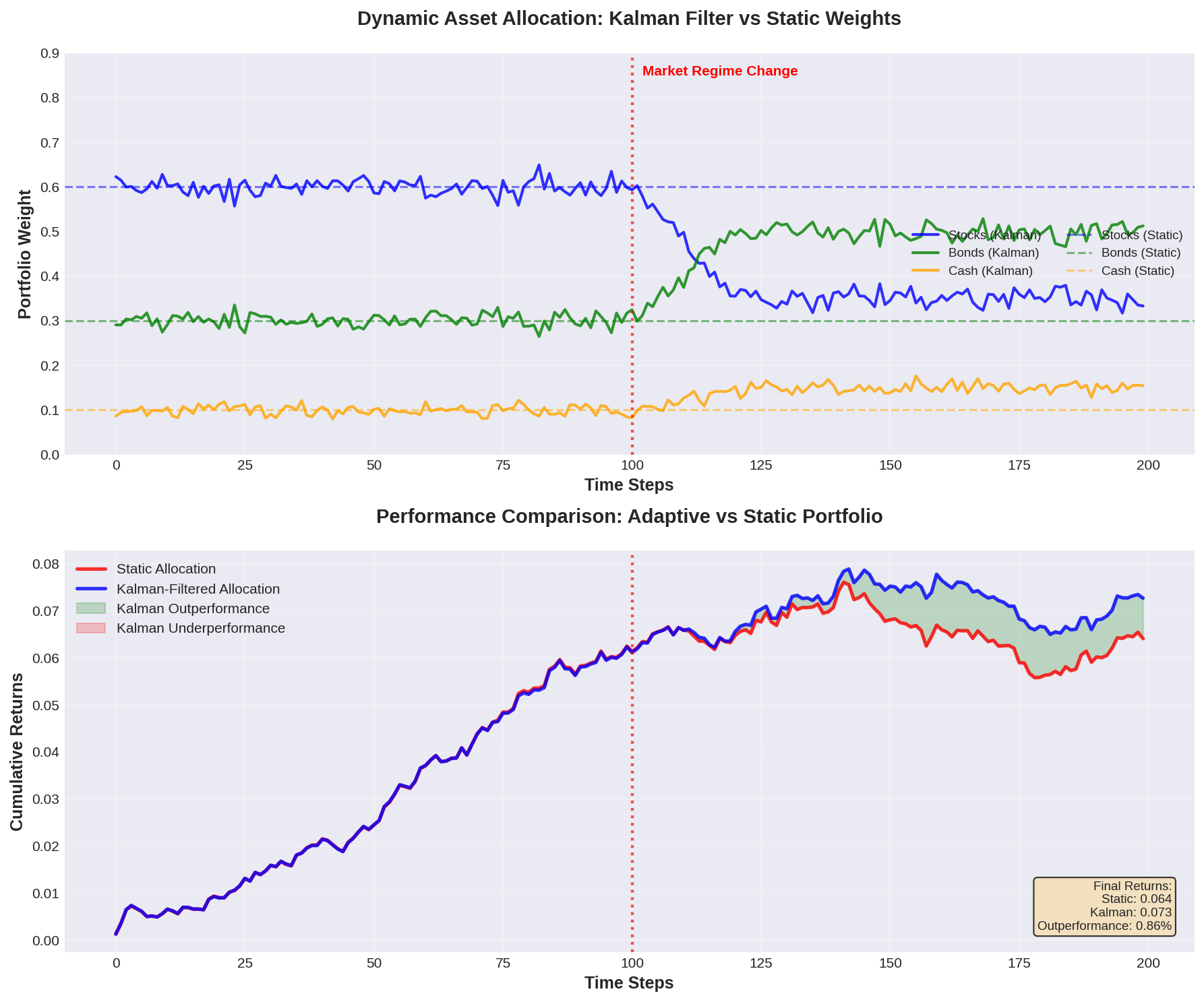
Out-of-sample backtesting should compare Kalman-filtered strategies against static benchmarks and rolling-window estimators. Key metrics include Sharpe ratio, maximum drawdown, and turnover costs. The filter's advantage typically manifests in faster adaptation to regime changes and reduced estimation error compared to simple historical averaging.

Computational efficiency matters for high-frequency applications. Standard Kalman filtering scales as O(n³) in the state dimension, but specialized algorithms exploit structure in financial covariance matrices to achieve near-linear scaling for large portfolios.

Conclusion

Kalman filtering transforms dynamic asset allocation from an ad-hoc rebalancing exercise into a principled statistical framework. By explicitly modeling the evolution of unobservable market parameters and optimally fusing prior knowledge with new data, it enables portfolio strategies that adapt systematically to changing conditions while managing estimation uncertainty. Modern extensions handle the nonlinearities and time-varying dynamics inherent in financial markets, making Kalman filtering an essential tool for quantitative portfolio management.

Implementing Kalman Filtering for Dynamic Asset Allocation Models

The State-Space Framework for Financial Modeling

Implementation Strategy for Portfolio Applications

Advanced Extensions and Practical Considerations

Performance Monitoring and Validation

Conclusion

Further Reading