
Implementing the Heston Stochastic Volatility Model for Equity Derivatives Pricing
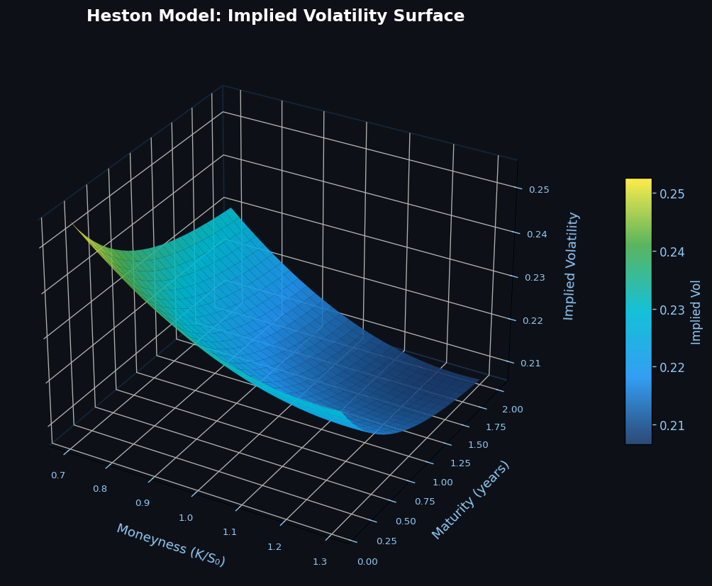
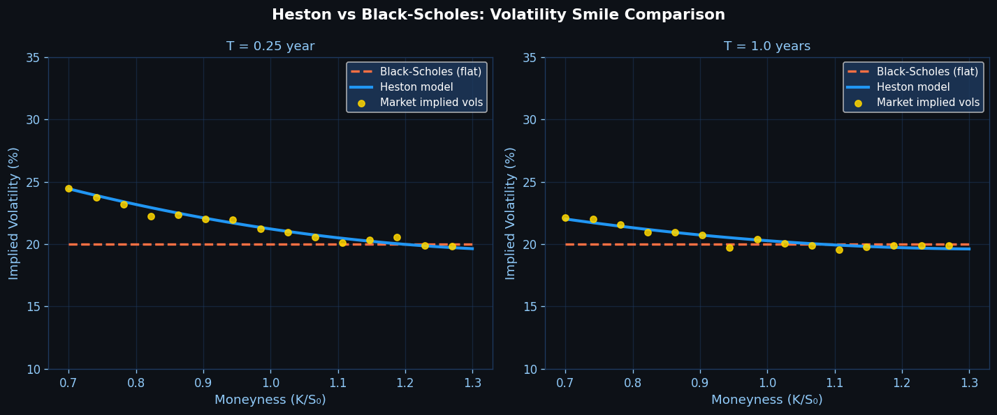
The Black-Scholes model's assumption of constant volatility has long been recognized as a critical limitation in practice. Real equity markets exhibit the volatility smile — implied volatilities that vary systematically with strike and maturity — a phenomenon that constant-volatility models cannot reproduce. The Heston (1993) stochastic volatility model addresses this by allowing variance itself to follow a mean-reverting stochastic process, making it the most widely deployed stochastic volatility framework in equity derivatives desks worldwide.
This article covers the Heston model's mathematical structure, calibration to market implied volatility surfaces, semi-analytical pricing via the characteristic function, and Monte Carlo simulation with full-truncation discretization — with practical Python implementations throughout.
The Heston Model: Mathematical Structure
Under the risk-neutral measure, the Heston model specifies joint dynamics for the asset price $S_t$ and its instantaneous variance $v_t$:
$$dS_t = r S_t \, dt + \sqrt{v_t} \, S_t \, dW_t^S$$
$$dv_t = \kappa(\theta - v_t) \, dt + \sigma \sqrt{v_t} \, dW_t^v$$
$$dW_t^S \, dW_t^v = \rho \, dt$$
The five parameters carry clear financial interpretations:
| Parameter | Symbol | Typical Range | Interpretation |
|---|---|---|---|
| Mean reversion speed | $\kappa$ | 1–10 | Rate at which variance reverts to $\theta$ |
| Long-run variance | $\theta$ | 0.01–0.25 | Equilibrium variance level |
| Vol-of-vol | $\sigma$ | 0.1–1.5 | Volatility of the variance process |
| Correlation | $\rho$ | −0.9 to −0.1 | Leverage effect (typically negative for equities) |
| Initial variance | $v_0$ | 0.01–0.5 | Current instantaneous variance |
The Feller condition $2\kappa\theta > \sigma^2$ ensures the variance process remains strictly positive almost surely. In practice, calibrated parameters often violate this condition, requiring careful discretization in Monte Carlo.
Semi-Analytical Pricing via the Characteristic Function
The Heston model's key advantage is the availability of a semi-analytical formula for European options through the characteristic function of $\ln S_T$. The option price is computed via Fourier inversion:
$$C(K, T) = S_0 P_1 - K e^{-rT} P_2$$
where $P_1$ and $P_2$ are risk-neutral probabilities obtained by integrating the characteristic function $\phi(u; t, S, v)$:
$$\phi(u; \tau, v_0) = \exp!\left(C(\tau, u) + D(\tau, u) v_0 + iu \ln S_0\right)$$
with closed-form expressions for $C$ and $D$ (see Heston 1993, or the numerically stable Albrecher et al. 2007 formulation).
import numpy as np
from scipy.integrate import quad

def heston_char_func(u, S0, v0, kappa, theta, sigma, rho, r, tau):
    """Heston characteristic function (Albrecher et al. stable form)."""
    xi = kappa - sigma * rho * 1j * u
    d  = np.sqrt(xi**2 + sigma**2 * (u**2 + 1j * u))
    g2 = (xi - d) / (xi + d)
    C  = (r * 1j * u * tau
          + (kappa * theta / sigma**2)
          * ((xi - d) * tau - 2 * np.log((1 - g2 * np.exp(-d * tau)) / (1 - g2))))
    D  = ((xi - d) / sigma**2) * (1 - np.exp(-d * tau)) / (1 - g2 * np.exp(-d * tau))
    return np.exp(C + D * v0 + 1j * u * np.log(S0))

def heston_call_price(S0, K, r, tau, v0, kappa, theta, sigma, rho):
    """European call price via Heston semi-analytical formula."""
    def integrand(u, j):
        cf = heston_char_func(u - 1j * (j == 1), S0, v0, kappa, theta, sigma, rho, r, tau)
        cf0 = heston_char_func(-1j * (j == 1), S0, v0, kappa, theta, sigma, rho, r, tau)
        return np.real(np.exp(-1j * u * np.log(K)) * cf / (1j * u * cf0))

    P1 = 0.5 + (1 / np.pi) * quad(integrand, 1e-8, 200, args=(1,))[0]
    P2 = 0.5 + (1 / np.pi) * quad(integrand, 1e-8, 200, args=(0,))[0]
    return S0 * P1 - K * np.exp(-r * tau) * P2
This approach prices a single European option in milliseconds, making it practical for real-time calibration.
Calibration to the Implied Volatility Surface
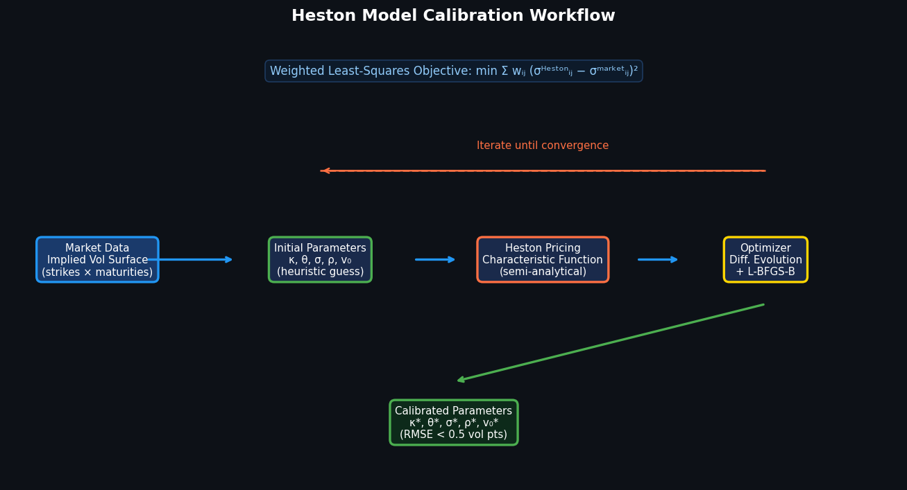
Calibration fits the five Heston parameters to market-observed implied volatilities across a grid of strikes and maturities. The standard approach minimizes a weighted least-squares objective:
$$\min_{\kappa, \theta, \sigma, \rho, v0} \sum{i,j} w{ij} \left(\sigma^{\text{Heston}}{ij} - \sigma^{\text{market}}_{ij}\right)^2$$
Practical calibration tips:
- Use relative weights proportional to option liquidity (bid-ask spread inverse) to avoid over-fitting illiquid wings.
- Regularize with a penalty on $\sigma$ (vol-of-vol) to prevent extreme curvature.
- Initialize with $\rho \approx -0.7$, $\kappa \approx 2$, $\theta \approx v_0 \approx \text{ATM variance}$, $\sigma \approx 0.5$.
- Apply bounds: $\kappa \in [0.1, 20]$, $\theta \in [0.001, 1]$, $\sigma \in [0.01, 2]$, $\rho \in [-0.99, -0.01]$, $v_0 \in [0.001, 1]$.
- Use global optimizers (differential evolution, CMA-ES) followed by local refinement (L-BFGS-B) to avoid local minima.
A well-calibrated Heston model typically achieves implied volatility fit errors below 0.5 vol points across liquid strikes (80%–120% moneyness) for maturities from 1 month to 2 years.
Monte Carlo Simulation with Full-Truncation Discretization
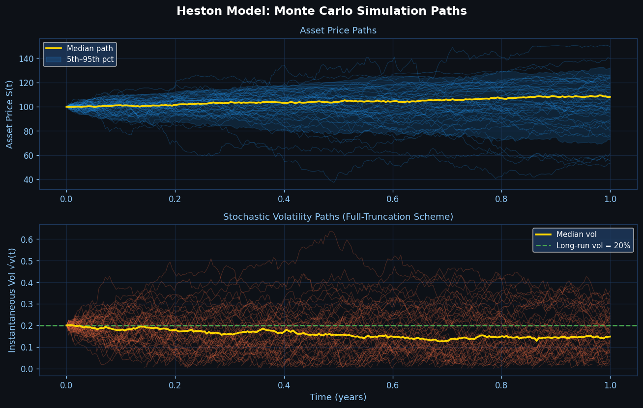
When the Feller condition is violated, naive Euler-Maruyama discretization of the variance process can produce negative values. The full-truncation (FT) scheme (Lord et al. 2010) is the recommended approach:
$$v_{t+\Delta t}^+ = \max(vt, 0)$$
$$v{t+\Delta t} = v_t + \kappa(\theta - v_t^+)\Delta t + \sigma\sqrt{v_t^+ \Delta t}\, Z_v$$
def heston_mc(S0, v0, kappa, theta, sigma, rho, r, T, n_steps, n_paths, seed=42):
    """Heston Monte Carlo with full-truncation scheme."""
    rng = np.random.default_rng(seed)
    dt  = T / n_steps
    S   = np.full(n_paths, S0, dtype=float)
    v   = np.full(n_paths, v0, dtype=float)

    for _ in range(n_steps):
        Z1 = rng.standard_normal(n_paths)
        Z2 = rho * Z1 + np.sqrt(1 - rho**2) * rng.standard_normal(n_paths)
        v_pos = np.maximum(v, 0)
        v    += kappa * (theta - v_pos) * dt + sigma * np.sqrt(v_pos * dt) * Z2
        S    *= np.exp((r - 0.5 * v_pos) * dt + np.sqrt(v_pos * dt) * Z1)

    return S, v
For production use, apply antithetic variates (negate both $Z_1$ and $Z_2$) and control variates (using the geometric Brownian motion price as a control) to reduce variance by 60–80% without additional paths.
Practical Considerations and Extensions
Calibration stability: The Heston surface is not always uniquely identified — particularly $\kappa$ and $\theta$ can be nearly collinear. Consider fixing $\kappa$ from time-series estimation and calibrating only the remaining four parameters.
Heston-Hull-White: For interest rate-sensitive equity products (e.g., equity-linked notes), extend to the Heston-Hull-White model, which adds a stochastic short rate correlated with both $S$ and $v$.
Rough Heston: Recent empirical work (El Euch & Rosenbaum 2019) shows that replacing the Brownian driver of variance with a fractional Brownian motion (Hurst exponent $H \approx 0.1$) dramatically improves short-maturity smile fit. The rough Heston retains a semi-analytical characteristic function via fractional Riccati equations.
GPU acceleration: For large-scale calibration or exotic pricing, vectorize the Monte Carlo across GPU threads using CuPy or JAX. A 100,000-path, 252-step simulation runs in under 0.5 seconds on a modern GPU versus ~15 seconds on CPU.
Further Reading
- Heston, S.L. (1993). A Closed-Form Solution for Options with Stochastic Volatility. Review of Financial Studies, 6(2), 327–343.
- Lord, R., Koekkoek, R., & Van Dijk, D. (2010). A Comparison of Biased Simulation Schemes for Stochastic Volatility Models. Quantitative Finance, 10(2), 177–194.
- Albrecher, H., Mayer, P., Schachermayer, W., & Teichmann, J. (2007). The Moment Formula for Implied Volatility at Extreme Strikes. Mathematical Finance, 17(2), 169–176.
- QuantLib Python documentation — includes Heston model calibration examples
- SSRN: Rough Heston Model — El Euch & Rosenbaum (2019)
The Heston model remains the practitioner's workhorse for equity derivatives precisely because it balances analytical tractability with realistic volatility dynamics. Mastering its calibration and simulation is an essential skill for any quantitative analyst working with options, structured products, or risk management systems.