Hull-White One-Factor Model: Implementation Guide for Interest Rate Derivatives

Interest rate derivatives—caps, floors, swaptions, and callable bonds—require a model that can be calibrated to the current yield curve while producing realistic future rate dynamics. The Hull-White one-factor (HW1F) model remains the workhorse of fixed-income desks worldwide precisely because it achieves both goals: it fits today's term structure exactly and admits closed-form solutions for vanilla instruments, making it fast enough for real-time pricing and Monte Carlo scenario generation alike.

Why Hull-White Over Simpler Alternatives?

The classic Vasicek model produces analytically tractable bond prices but cannot match an arbitrary initial yield curve—a fatal flaw for derivatives pricing. The Cox-Ingersoll-Ross (CIR) model adds mean-reversion with non-negative rates but shares the same calibration limitation. Hull and White (1990) resolved this by introducing a time-dependent drift term θ(t) that is bootstrapped directly from the observed zero-coupon curve:

dr(t) = [θ(t) − a·r(t)] dt + σ dW(t)

Here, a is the mean-reversion speed, σ is the short-rate volatility, and θ(t) is determined analytically from the market discount factors. The result is a Gaussian short-rate model that is arbitrage-free by construction.

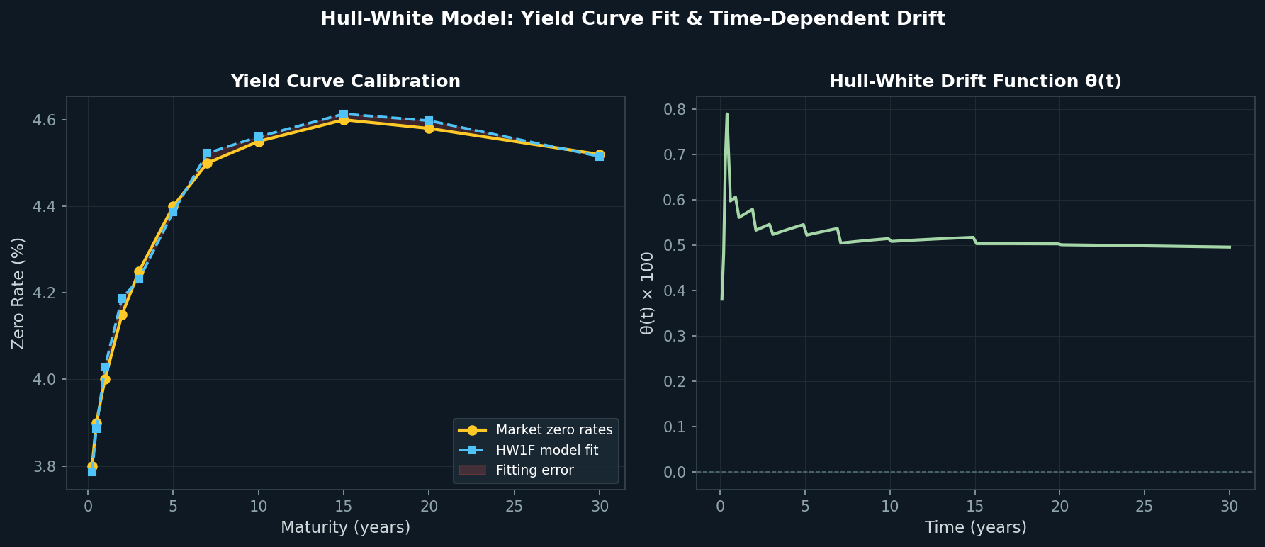
Calibrating θ(t) from the Yield Curve

Given a set of market zero rates Z(0, T) for maturities T₁ < T₂ < … < Tₙ, the Hull-White drift function is:

θ(t) = ∂f(0,t)/∂t + a·f(0,t) + σ²/(2a) · (1 − e^{−2at})

where f(0, t) is the instantaneous forward rate implied by the market curve. In practice, practitioners discretize this on a fine time grid and interpolate between market pillars. A robust implementation in Python using QuantLib looks like this:

import QuantLib as ql

# Market data
calendar = ql.TARGET()
today = ql.Date(13, 6, 2026)
ql.Settings.instance().evaluationDate = today

# Build flat or bootstrapped yield curve
flat_rate = ql.QuoteHandle(ql.SimpleQuote(0.04))
day_count = ql.Actual365Fixed()
term_structure = ql.YieldTermStructureHandle(
    ql.FlatForward(today, flat_rate, day_count)
)

# Hull-White model: a=0.10, sigma=0.01
hw_model = ql.HullWhite(term_structure, a=0.10, sigma=0.01)

For a real desk application, replace FlatForward with a bootstrapped PiecewiseLogLinearDiscount curve built from deposit rates, FRAs, and swap quotes.

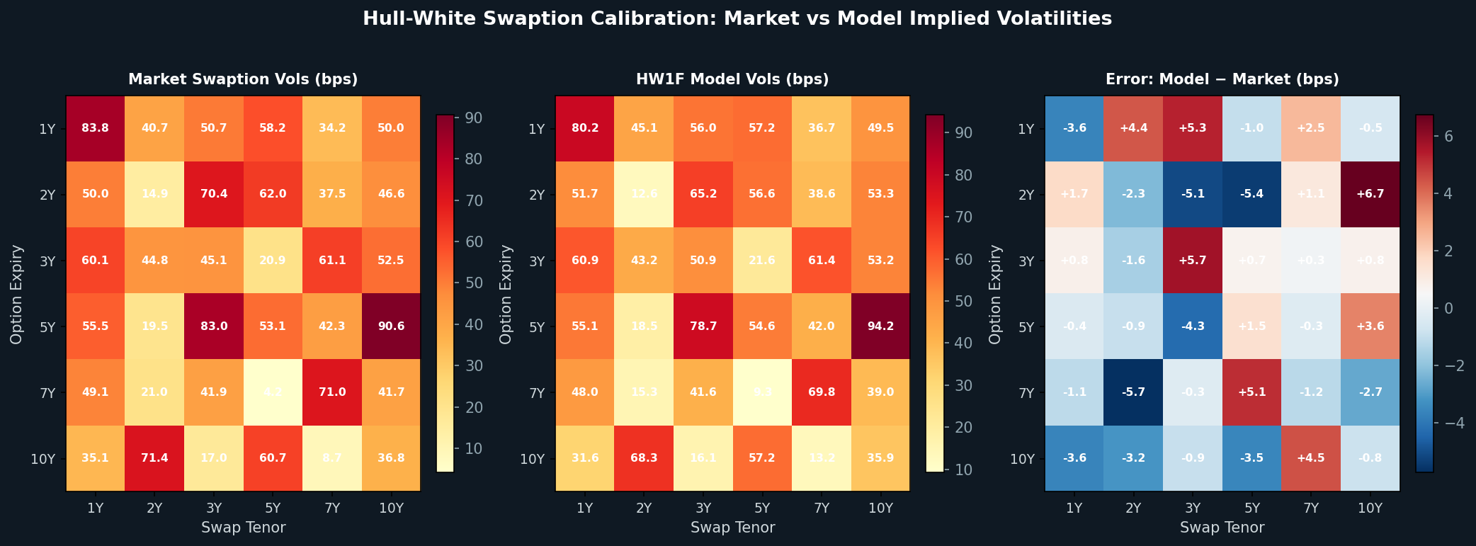
Calibrating a and σ to Swaption Volatilities

The parameters a and σ are calibrated by minimizing the sum of squared differences between model and market swaption implied volatilities. QuantLib's LevenbergMarquardt optimizer handles this efficiently:

swaption_helpers = []
for expiry, tenor, vol in market_swaptions:
    helper = ql.SwaptionHelper(
        ql.Period(expiry, ql.Years),
        ql.Period(tenor, ql.Years),
        ql.QuoteHandle(ql.SimpleQuote(vol)),
        index,
        ql.Period(1, ql.Years),
        day_count,
        day_count,
        term_structure
    )
    helper.setPricingEngine(ql.JamshidianSwaptionEngine(hw_model))
    swaption_helpers.append(helper)

optimizer = ql.LevenbergMarquardt()
end_criteria = ql.EndCriteria(1000, 100, 1e-8, 1e-8, 1e-8)
hw_model.calibrate(swaption_helpers, optimizer, end_criteria)

print(f"Calibrated a={hw_model.params()[0]:.4f}, σ={hw_model.params()[1]:.4f}")

A well-calibrated model typically achieves a root-mean-square error below 5 basis points on the ATM swaption grid.

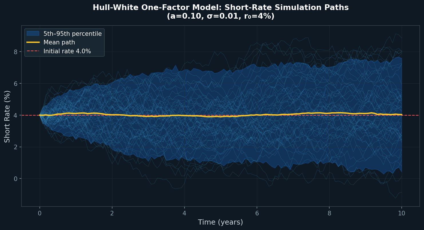
Monte Carlo Simulation of Short-Rate Paths

Once calibrated, the HW1F model generates short-rate scenarios for CVA, XVA, and scenario analysis. The exact discretization avoids numerical drift:

import numpy as np

def hw_simulate(a, sigma, theta_func, r0, T, n_steps, n_paths, seed=42):
    """Exact discretization of Hull-White short rate."""
    rng = np.random.default_rng(seed)
    dt = T / n_steps
    paths = np.zeros((n_paths, n_steps + 1))
    paths[:, 0] = r0

    for i in range(n_steps):
        t = i * dt
        theta = theta_func(t)
        mean = paths[:, i] * np.exp(-a * dt) + (theta / a) * (1 - np.exp(-a * dt))
        var = (sigma**2 / (2 * a)) * (1 - np.exp(-2 * a * dt))
        paths[:, i + 1] = mean + np.sqrt(var) * rng.standard_normal(n_paths)

    return paths

Using antithetic variates or Sobol quasi-random sequences (available via scipy.stats.qmc) can reduce the standard error of discount factor estimates by 30–50% compared to plain Monte Carlo.

Hull-White Model yield curve calibration and time-dependent drift function θ(t)

Pricing Zero-Coupon Bond Options (Caps and Floors)

A key advantage of the HW1F model is the closed-form bond option price, which underpins cap and floor valuation. For a call on a zero-coupon bond P(T, S) with strike K:

Price = P(0,S)·N(h) − K·P(0,T)·N(h − σ_P)

where σ_P is the bond option volatility derived analytically from a, σ, T, and S. This makes cap/floor pricing nearly instantaneous—critical for Greeks computation via bump-and-reprice.

Hull-White swaption calibration heatmap comparing market and model implied volatilities

Practical Considerations for Production Use

Negative rates: The Gaussian nature of HW1F allows negative rates, which is a feature in EUR and JPY markets but requires careful handling of log-normal payoffs. Consider the shifted Black model for floor pricing when rates are near zero.

Multi-curve framework: Post-2008, OIS discounting and LIBOR/SOFR projection curves must be handled separately. Calibrate the HW1F model to OIS-discounted swaption prices and use a deterministic spread for the projection curve.

Numerical stability: When a is very small (< 0.01), the exponential terms approach 1 and numerical cancellation occurs. Apply L'Hôpital's rule or use the Taylor expansion (1 − e^{−aT})/a ≈ T − aT²/2 for small a.

Bermudan swaptions: For callable bonds and Bermudan swaptions, combine the HW1F model with a trinomial tree (QuantLib's TreeSwaptionEngine) or the Longstaff-Schwartz regression Monte Carlo approach for accurate early-exercise boundaries.

Further Resources

Hull, J. & White, A. (1990). Pricing Interest-Rate Derivative Securities. Review of Financial Studies, 3(4), 573–592.
QuantLib Documentation – Hull-White Model
QuantLib Python Cookbook
Brigo, D. & Mercurio, F. (2006). Interest Rate Models – Theory and Practice (2nd ed.). Springer Finance.
OpenGamma Strata – Interest Rate Calibration

The Hull-White one-factor model strikes an ideal balance between analytical tractability and market consistency. For teams building interest rate simulation infrastructure, mastering its calibration workflow and Monte Carlo discretization is an essential foundation before moving to more complex multi-factor or SABR-LMM frameworks.