MSC Nastran SOL 200: Gradient-Based Design Optimization for Structural Engineers

MSC Nastran's Solution Sequence 200 (SOL 200) is one of the most powerful yet underutilized capabilities in the structural simulation toolkit. While most engineers are familiar with Nastran's static (SOL 101), normal modes (SOL 103), and buckling (SOL 105) analyses, SOL 200 elevates the software from a passive analysis tool into an active design driver — automatically finding the optimal structural configuration that satisfies engineering constraints while minimizing or maximizing a defined objective.

What Is SOL 200?

SOL 200 is Nastran's integrated gradient-based design optimization solver. It couples finite element analysis with mathematical programming to iteratively adjust design variables — such as element thicknesses, cross-sectional dimensions, material properties, or even nodal coordinates — until the structure meets all specified constraints at the best possible objective value.

The optimization engine uses the Modified Method of Feasible Directions (MMFD) and the Sequential Linear Programming (SLP) algorithm, both of which rely on design sensitivity analysis (DSA) to compute how the objective and constraint functions change with respect to each design variable. This sensitivity information is computed analytically within Nastran, making it far more efficient than finite-difference-based approaches used by external optimization wrappers.

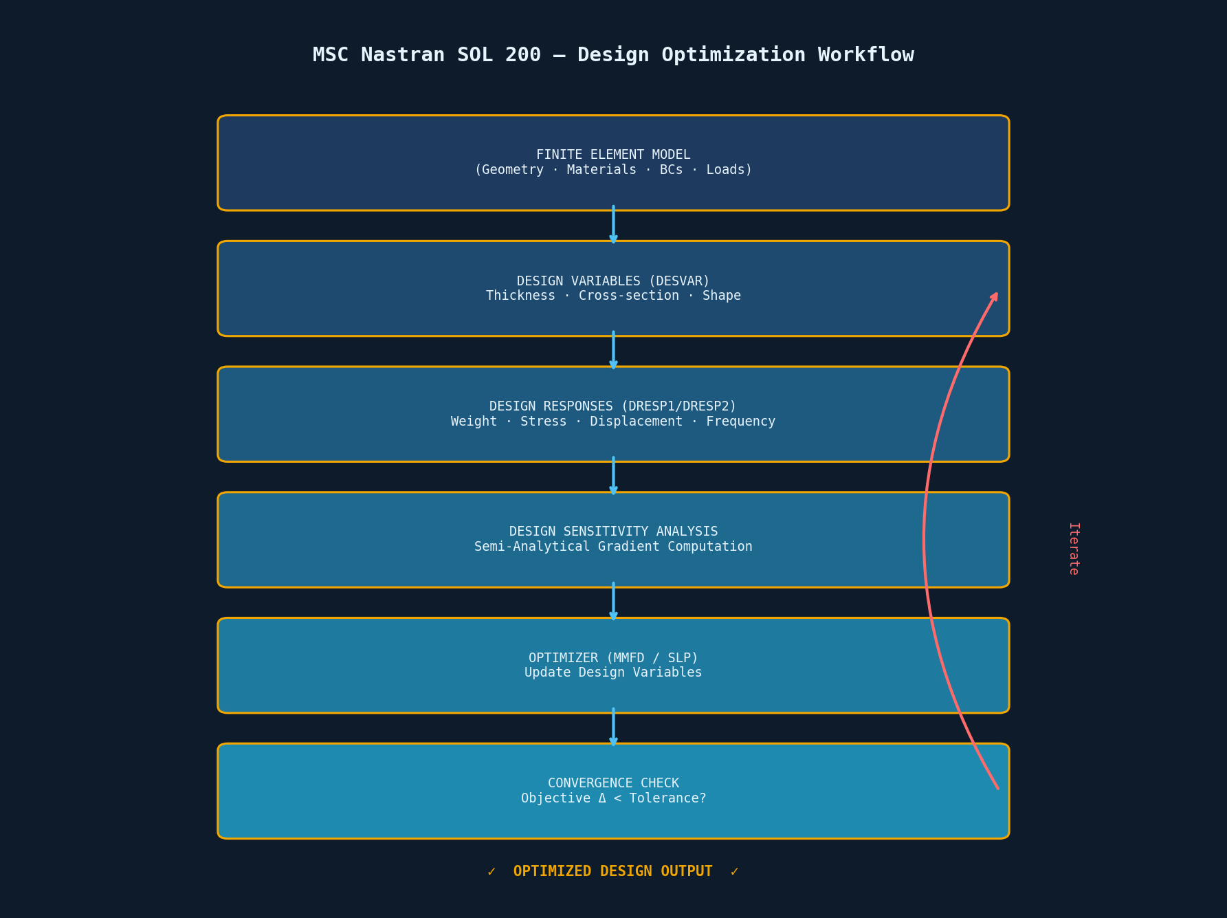
Key Components of a SOL 200 Model

A SOL 200 input deck extends a standard Nastran model with four additional bulk data sections:

1. Design Variables (DESVAR)

Each DESVAR entry defines a scalar design variable with initial, lower-bound, and upper-bound values. For example, a shell thickness optimization might define 20 independent thickness variables, each mapped to a group of elements via DVPREL1 or DVPREL2 property-to-design-variable relations.

DESVAR, 1, T_SKIN, 3.0, 0.5, 10.0
DVPREL1, 10, PSHELL, 101, T, , , ,
        , 1, 1.0

2. Design Responses (DRESP1 / DRESP2)

Responses are the quantities that appear in the objective or constraints. DRESP1 accesses native Nastran outputs directly — stress, displacement, frequency, weight, buckling factor — while DRESP2 allows user-defined algebraic combinations of DRESP1 quantities via DEQATN equations.

Common responses include:

• Weight (WEIGHT) — the most frequent objective
• Displacement (DISP) — for stiffness constraints
• Stress (STRESS) — for strength constraints
• Frequency (FREQ) — for dynamic stiffness or resonance avoidance
• Buckling load factor (LAMA) — for stability constraints

3. Design Constraints (DCONSTR)

DCONSTR entries bound each response between lower and upper limits. Multiple constraints can be grouped under a DCONADD entry and referenced by the optimization case control.

4. Objective Function (DESOBJ)

The case control command DESOBJ(MIN) = n or DESOBJ(MAX) = n designates which DRESP1/DRESP2 response ID is the objective. Minimizing structural weight subject to stress and displacement constraints is the canonical use case.

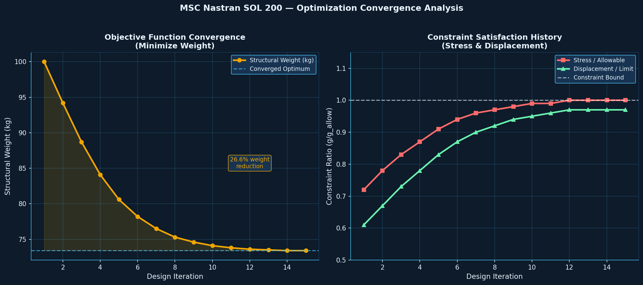
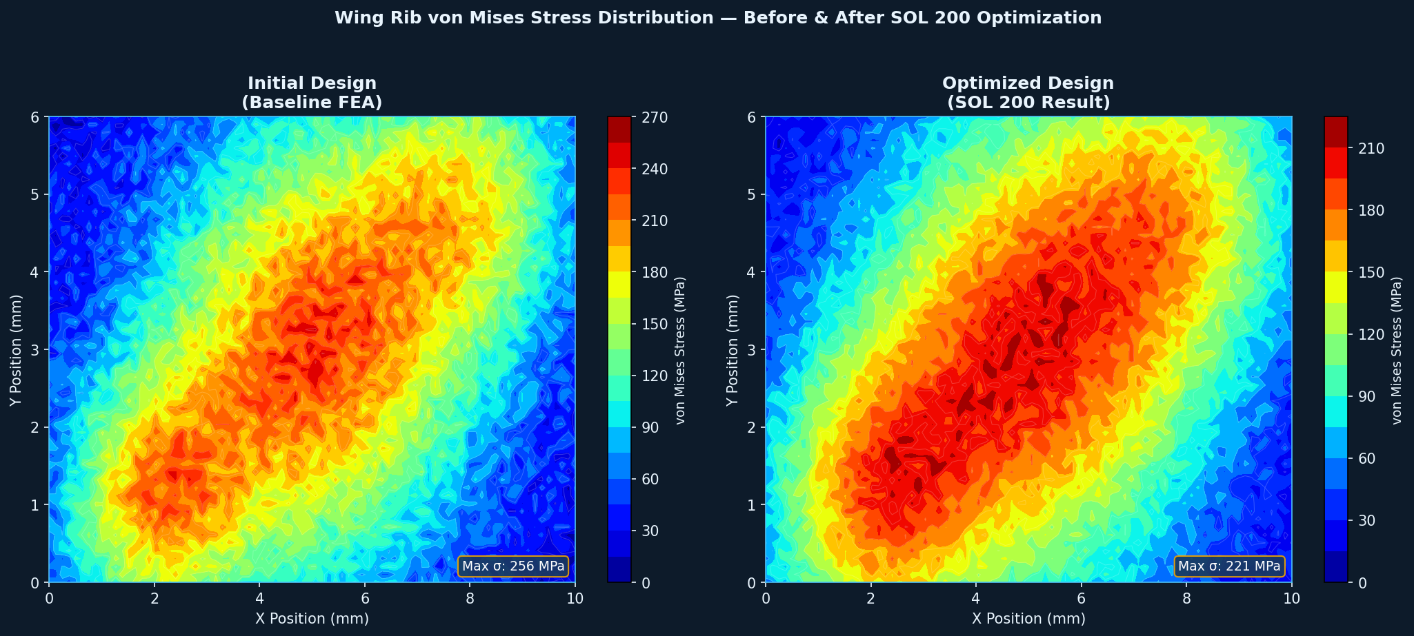
Practical Workflow: Wing Rib Thickness Optimization

Consider a simplified aircraft wing rib modeled with CQUAD4 shell elements. The goal is to minimize total mass while keeping von Mises stress below 250 MPa under a 2.5g maneuver load and limiting tip displacement to 15 mm.

Step 1 — Baseline Analysis: Run SOL 101 to verify the baseline model and identify the most highly stressed regions. This informs the grouping of design variables.

Step 2 — Variable Grouping: Rather than making every element an independent variable (which creates an ill-conditioned problem), group elements by structural role: spar caps, rib webs, skin panels. This reduces the design space to a manageable 10–30 variables.

Step 3 — Response Definition: Define DRESP1 entries for total weight, maximum von Mises stress per group (using STRESS with PTYPE=PSHELL), and tip displacement.

Step 4 — Constraint Tightening: Set stress upper bounds at 90% of the allowable (225 MPa) to provide a margin against manufacturing variability. Apply the displacement constraint as a hard upper bound.

Step 5 — Convergence Monitoring: SOL 200 outputs a DSCREN summary after each design cycle showing objective value, active constraints, and design variable changes. Convergence is typically achieved in 5–15 cycles for well-posed problems.

Design Sensitivity Analysis: The Engine Under the Hood

The efficiency of SOL 200 stems from its semi-analytical design sensitivity analysis. For each design variable, Nastran computes the partial derivative of every active response with respect to that variable by differentiating the finite element equations analytically — avoiding the 2N function evaluations required by finite differences (where N is the number of design variables).

For frequency responses, Nastran uses modal design sensitivity based on the eigenvector expansion, which is particularly efficient when only a few modes are active constraints. For stress responses, the sensitivity is computed via the adjoint method, requiring only one additional linear solve per load case regardless of the number of design variables.

Multi-Disciplinary Optimization with SOL 200

SOL 200 supports simultaneous optimization across multiple subcases — static, normal modes, and buckling — within a single run. This enables true multi-disciplinary structural optimization:

• Stiffness + Strength: Minimize weight subject to both displacement (stiffness) and stress (strength) constraints from static subcases
• Stiffness + Dynamics: Add frequency constraints to avoid resonance with known excitation frequencies
• Stiffness + Stability: Include buckling load factor constraints for thin-walled structures

The SUBCASE structure in the case control section allows each subcase to contribute its own set of responses and constraints to the unified optimization problem.

Topology Optimization via SOL 200 + ESLM

For concept-phase design, MSC Nastran also supports topology optimization through the Equivalent Static Load Method (ESLM) when paired with MSC's OptiStruct-compatible input format. However, for sizing and shape optimization of production-intent models, SOL 200's gradient-based approach delivers faster convergence and more interpretable results than density-based topology methods.

Limitations and Best Practices

Avoid over-constraining: Too many active constraints at the initial design point can cause the optimizer to oscillate. Start with the two or three most critical constraints and add others progressively.

Check sensitivity accuracy: Use the DSAPRT case control command to print sensitivity values and verify them against finite-difference checks for at least a subset of variables before trusting optimization results.

Discrete variables: SOL 200 is a continuous optimizer. For discrete thickness selections (e.g., standard gauge sheet metal), post-process the continuous optimum by rounding to the nearest available gauge and re-running a verification analysis.

Large models: For models exceeding ~500,000 DOF, consider using the PARAM,DSNOKD,1 option to skip sensitivity computation for non-design elements, significantly reducing runtime.

Integration with Pre/Post-Processing Tools

SOL 200 models can be set up and post-processed through:

• MSC Apex / Patran: Native SOL 200 setup wizards with graphical design variable definition
• Femap: Full SOL 200 support via the Optimization Manager module
• HyperMesh (Altair): Nastran optimization template with automated DESVAR/DRESP1 generation
• Python + pyNastran: Programmatic model generation and results parsing for parametric studies (pyNastran documentation)

Further Reading

• MSC Nastran Design Sensitivity and Optimization User's Guide — the definitive reference for all SOL 200 bulk data entries
• NASA Technical Memorandum on Structural Optimization — foundational theory behind gradient-based structural optimization
• MSC Software SOL 200 Webinar Series — practical tutorials covering automotive and aerospace applications
• pyNastran GitHub Repository — open-source Python library for reading, writing, and modifying Nastran input/output files

MSC Nastran SOL 200 represents a mature, production-proven approach to structural optimization that integrates seamlessly into existing FEA workflows. By leveraging analytical design sensitivity, multi-subcase optimization, and a rich library of structural responses, it enables engineers to move beyond trial-and-error design iteration toward mathematically rigorous, constraint-driven optimization — delivering lighter, stiffer, and more reliable structures in fewer analysis cycles.