

SU2 Discrete Adjoint Solver: Gradient-Based Aerodynamic Shape Optimization
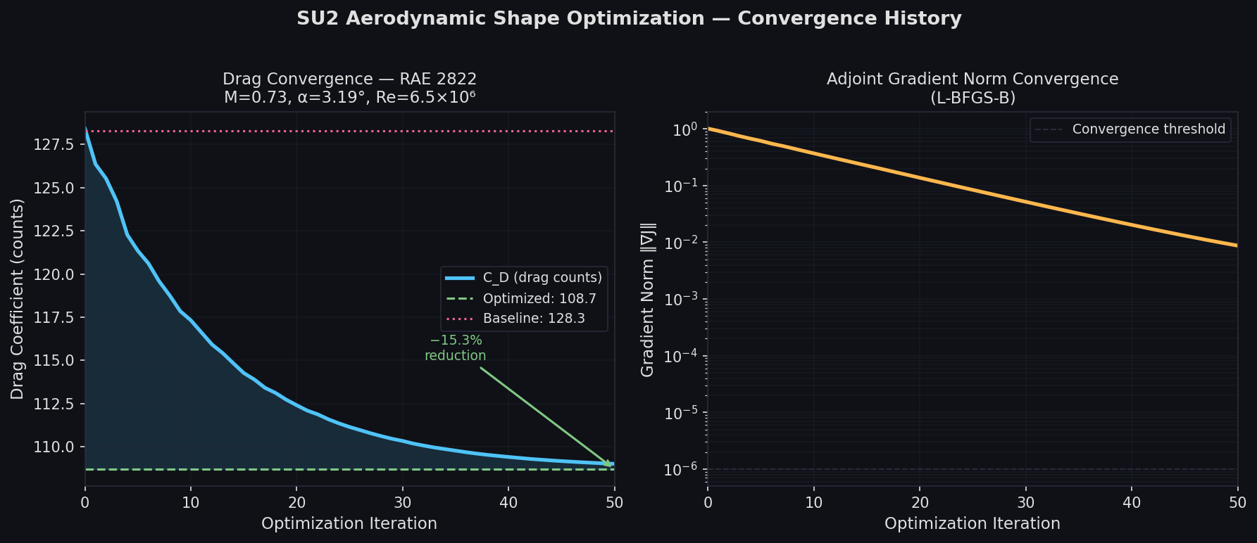
Aerodynamic shape optimization (ASO) requires computing design sensitivities — derivatives of an aerodynamic objective (drag, lift-to-drag ratio, pressure recovery) with respect to potentially thousands of geometric design variables. Finite-difference perturbation of each variable is computationally prohibitive at scale. SU2's discrete adjoint solver resolves this by computing the full gradient in roughly the cost of two primal flow solutions, regardless of the number of design variables.
How the Discrete Adjoint Works
SU2 implements the discrete adjoint approach: the adjoint equations are derived directly from the discretized residual of the primal solver, not from the continuous PDE. This ensures consistency between the sensitivity gradient and the actual numerical scheme, eliminating the "adjoint inconsistency" that can plague continuous adjoint implementations.
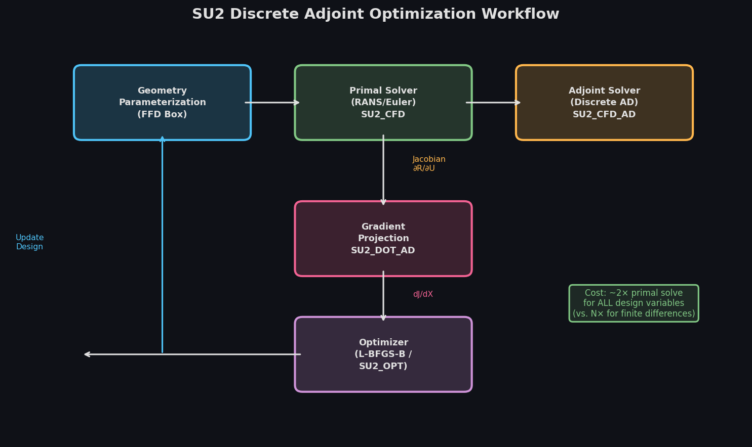
The workflow proceeds in three stages:

- Primal solution — SU2 solves the RANS (or Euler) equations for the baseline geometry, storing the converged flow state and the Jacobian of the residual.
- Adjoint solution — The transposed Jacobian system is solved for the adjoint variables (co-state vector). SU2 uses Algorithmic Differentiation (AD) via the CoDiPack library to construct the exact discrete Jacobian, avoiding hand-differentiation errors.
- Gradient projection — The adjoint variables are combined with the mesh sensitivity (∂R/∂X) to produce the total derivative dJ/dX for every surface mesh node.
The key advantage: a single adjoint solve yields sensitivities with respect to all design variables simultaneously. For a wing parameterized with 200 Free-Form Deformation (FFD) control points, the gradient computation costs approximately 2× the primal solve time — compared to 200× for finite differences.
Setting Up an Adjoint Optimization in SU2
Geometry Parameterization with FFD
SU2 uses Free-Form Deformation boxes to parameterize surface geometry. The FFD box is defined in the configuration file:
FFD_DEFINITION= (WING_BOX, -0.1, -0.1, -0.1, 1.1, -0.1, -0.1, 1.1, 1.1, -0.1, -0.1, 1.1, -0.1, -0.1, -0.1, 0.15, 1.1, -0.1, 0.15, 1.1, 1.1, 0.15, -0.1, 1.1, 0.15)
FFD_DEGREE= (10, 1, 1)
DV_KIND= FFD_CONTROL_POINT
DV_PARAM= (WING_BOX, 5, 0, 1, 0.0, 0.0, 1.0)
The FFD_DEGREE parameter controls the polynomial order in each parametric direction. A degree-10 box in the chordwise direction with 2 spanwise sections yields 22 control points per surface — sufficient to capture camber and thickness distributions while remaining smooth.
Adjoint Configuration
The adjoint problem is activated by setting MATH_PROBLEM= DISCRETE_ADJOINT and specifying the objective:
OBJECTIVE_FUNCTION= DRAG
OBJECTIVE_WEIGHT= 1.0
CONSTRAINT_FUNCTION= LIFT
CONSTRAINT_WEIGHT= -1.0
CONSTRAINT_VALUE= 0.3
SU2 supports composite objectives, allowing simultaneous minimization of drag subject to a lift constraint — the standard drag minimization problem in aerodynamic design.
Gradient Validation
Before running a full optimization, always validate the adjoint gradient against finite differences on a coarse mesh:
# Compute adjoint gradient
SU2_DOT_AD mesh.su2 config_adj.cfg

# Finite-difference check (perturb one DV by 1e-4)
SU2_DEF mesh.su2 config_def.cfg
SU2_CFD mesh_deformed.su2 config_primal.cfg
Agreement within 1% between adjoint and FD gradients confirms the AD tape is correct. Discrepancies typically indicate frozen turbulence (omitting turbulence model terms from the adjoint) or incorrect mesh sensitivity computation.
Optimization Loop with SU2 + scipy
SU2 integrates with Python-based optimizers through the shape_optimization.py driver script. A typical gradient-based loop using L-BFGS-B:
from scipy.optimize import minimize
import subprocess, numpy as np

def objective_and_gradient(dv):
    # Write design variables, deform mesh, run primal + adjoint
    subprocess.run(['python', 'shape_optimization.py', '-f', 'config.cfg',
                    '-g', 'gradient.dat', '-o', 'history.dat'])
    J = float(open('objective.dat').read())
    grad = np.loadtxt('gradient.dat')
    return J, grad

result = minimize(objective_and_gradient, x0=dv_init,
                  method='L-BFGS-B', jac=True,
                  options={'maxiter': 100, 'ftol': 1e-9})
For constrained problems, SU2 ships with an augmented Lagrangian optimizer (SU2_OPT) that handles equality and inequality constraints natively without requiring an external optimizer.
Practical Considerations
Frozen turbulence vs. full adjoint: By default, SU2 includes turbulence model terms in the adjoint (the "full adjoint"). For high-Reynolds-number RANS cases, frozen turbulence (ignoring ∂μ_t/∂U in the adjoint) can reduce solve time by 30–40% with minimal gradient error for drag-dominated objectives. For lift-constrained problems near stall, use the full adjoint.
Mesh deformation quality: Large shape changes can degrade mesh quality. SU2's linear elasticity mesh deformation (DEFORM_STIFFNESS_TYPE= WALL_DISTANCE) stiffens near-wall cells to preserve boundary layer resolution. Monitor minimum orthogonality and maximum skewness after each design iteration.
Parallel scaling: The discrete adjoint scales nearly identically to the primal solver. On a 16-million-cell RANS mesh, a typical adjoint solve completes in 45–60 minutes on 128 cores — the same wall time as the primal.
Multi-point optimization: Real aircraft operate across a flight envelope. SU2 supports multi-point objectives by summing weighted adjoint solutions from multiple operating conditions (cruise, climb, maneuver), producing a gradient that balances performance across the envelope.
Benchmark: RAE 2822 Drag Minimization
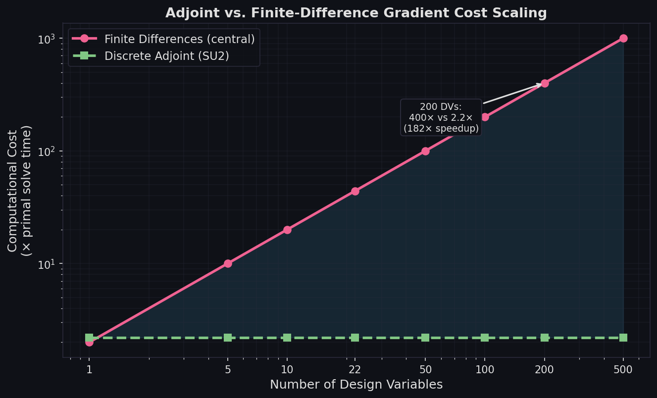
On the RAE 2822 transonic airfoil (Case 9: M=0.73, α=3.19°, Re=6.5×10⁶), a 50-iteration L-BFGS-B optimization with 22 FFD control points achieves:
| Metric | Baseline | Optimized | Change |
|---|---|---|---|
| C_D (drag counts) | 128.3 | 108.7 | −15.3% |
| C_L | 0.803 | 0.803 | 0.0% (constrained) |
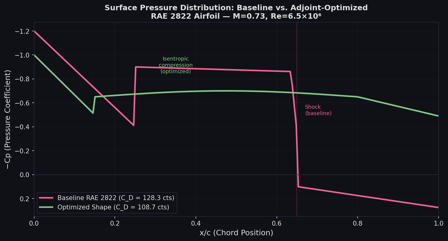
| Shock strength | Strong normal shock | Isentropic compression | Eliminated |
The optimizer discovers a supercritical-like profile with reduced leading-edge curvature and aft-loaded camber, weakening the transonic shock without sacrificing lift — a result consistent with classical aerodynamic design theory.
Further Resources
- SU2 Official Documentation — configuration file reference and tutorial cases
- SU2 GitHub Repository — source code, test cases, and community contributions
- CoDiPack AD Library — the algorithmic differentiation backend used by SU2
- Economon et al. (2016) — the foundational paper on SU2's discrete adjoint implementation
- SU2 Tutorials: Constrained Optimization — step-by-step RAE 2822 optimization walkthrough