VISSIM COM API: Automating Microscopic Traffic Simulation Workflows with Python

Transportation engineers increasingly rely on scripted automation to run large parameter sweeps, calibrate models against field data, and integrate traffic simulation into broader digital-twin pipelines. PTV VISSIM's Component Object Model (COM) API provides a programmatic interface that unlocks this level of automation—yet many practitioners still drive the tool exclusively through its graphical interface. This article examines the COM API in depth, covering its architecture, practical Python integration patterns, and real-world use cases that go well beyond what the GUI alone can achieve.

What Is the VISSIM COM API?

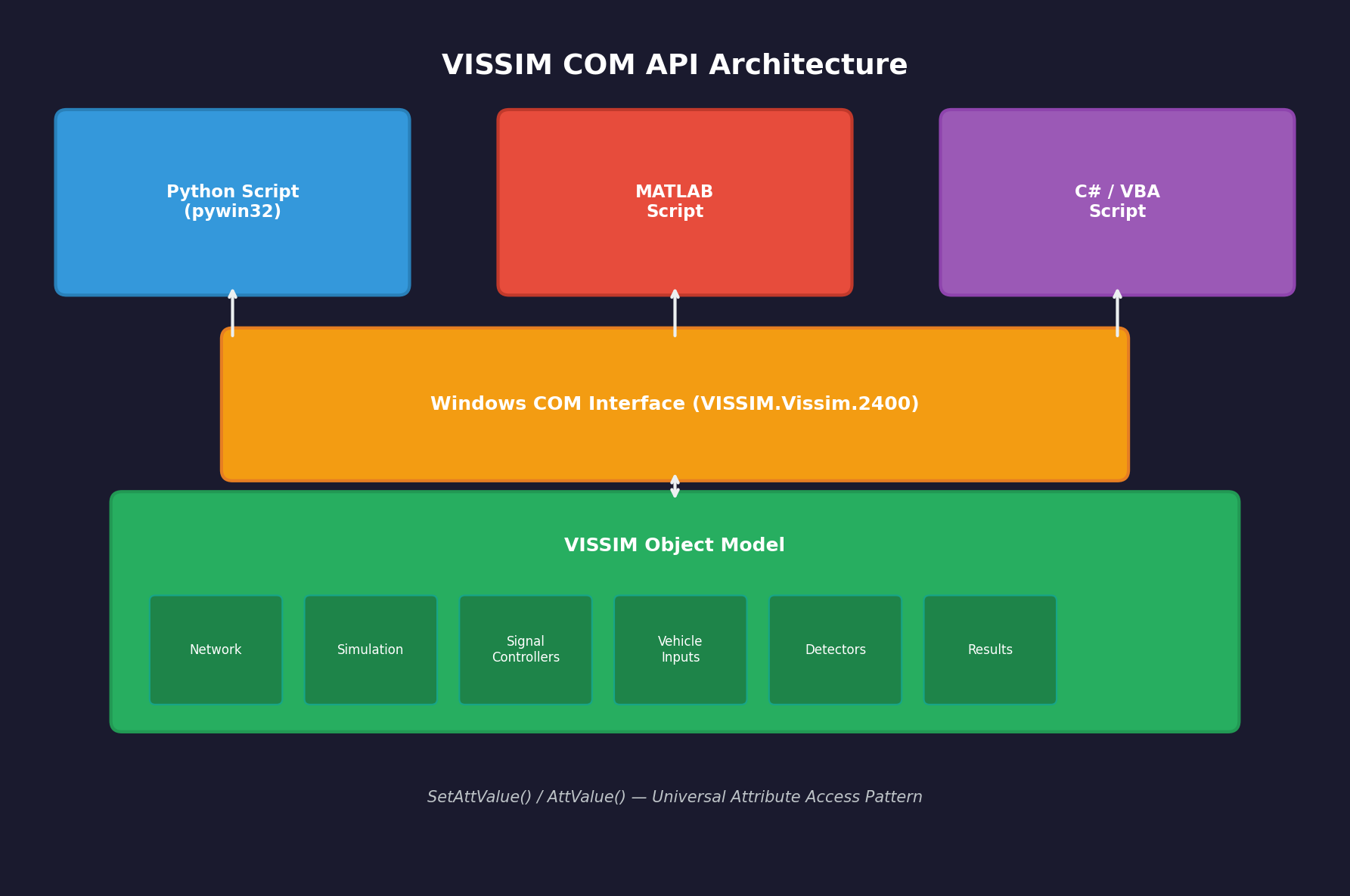
VISSIM exposes a Windows COM server that any COM-capable language—Python (via pywin32), MATLAB, C#, or VBA—can connect to at runtime. The API surface mirrors the VISSIM object model: networks, vehicle inputs, signal controllers, detectors, data collections, and simulation runs are all first-class objects you can read and write programmatically. Because the connection is live, you can modify network parameters between simulation runs without reloading the project, making iterative optimization loops orders of magnitude faster than manual GUI workflows.

The API is documented in the VISSIM COM Interface Manual (shipped with each VISSIM installation under \Doc\) and is versioned alongside the main product—scripts written for VISSIM 2023 will generally work on 2024 with minor namespace adjustments.

Connecting from Python

import win32com.client as com

# Attach to a running VISSIM instance or launch a new one
vissim = com.Dispatch("VISSIM.Vissim.2400")   # version suffix matches your install
vissim.LoadNet(r"C:\Projects\downtown_grid\downtown.inpx")
vissim.LoadLayout(r"C:\Projects\downtown_grid\downtown.layx")

sim = vissim.Simulation
sim.SetAttValue("SimPeriod", 3600)   # 1-hour simulation
sim.SetAttValue("RandSeed", 42)
sim.RunContinuous()

The SetAttValue / AttValue pattern is universal across the object model. Every VISSIM attribute—vehicle speed distributions, signal phase durations, routing decisions—is accessible through this pair of methods, making the API highly consistent once you understand the naming conventions.

Practical Use Case 1: Automated Signal Timing Optimization

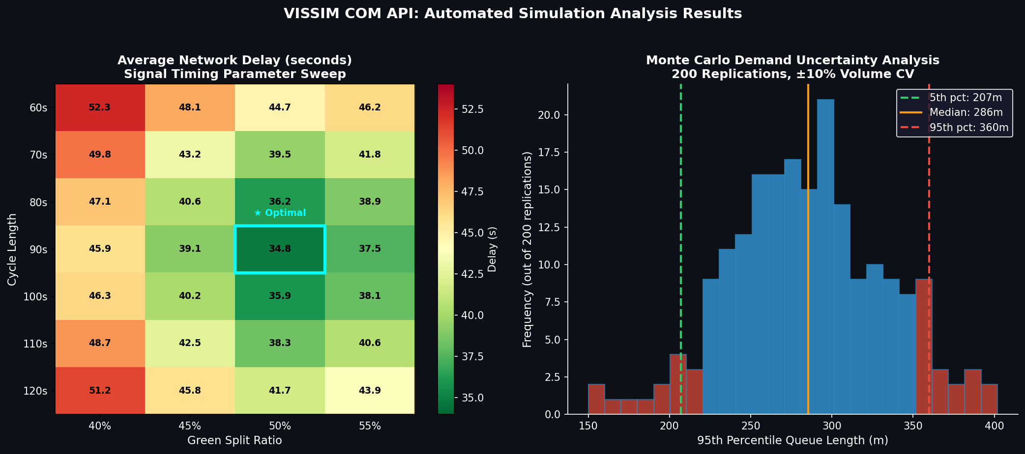
A common workflow is to sweep signal cycle lengths and green-split ratios across a corridor and record network-level performance metrics. The COM API makes this a straightforward nested loop:

net = vissim.Net
sig_controllers = net.SignalControllers

results = []
for cycle in range(60, 121, 10):          # 60 s to 120 s in 10-s steps
    for green_frac in [0.40, 0.45, 0.50, 0.55]:
        # Update all fixed-time controllers
        for sc in sig_controllers:
            for sg in sc.SGs:
                sg.SetAttValue("GreenTime", cycle * green_frac)
                sg.SetAttValue("CycleTime", cycle)

        sim.SetAttValue("RandSeed", 42)
        sim.RunContinuous()

        # Collect delay from all vehicle travel time measurements
        avg_delay = net.VehicleTravelTimeMeasurements.ItemByKey(1).AttValue("TravTm(Current,Last,All)")
        results.append({"cycle": cycle, "green_frac": green_frac, "avg_delay": avg_delay})

import pandas as pd
df = pd.DataFrame(results)
df.to_csv("signal_sweep_results.csv", index=False)

This 30-run sweep completes in minutes rather than the hours it would take to configure and execute manually—and the results feed directly into a Pareto-front analysis or a gradient-free optimizer such as scipy.optimize.differential_evolution.

Practical Use Case 2: Monte Carlo Demand Uncertainty Analysis

Traffic demand forecasts carry inherent uncertainty. The COM API enables Monte Carlo analysis by perturbing vehicle input volumes across hundreds of replications:

import numpy as np

vehicle_inputs = vissim.Net.VehicleInputs
base_volumes = {vi.AttValue("No"): vi.AttValue("Volume(1)") for vi in vehicle_inputs}

for rep in range(200):
    for vi in vehicle_inputs:
        no = vi.AttValue("No")
        noisy_vol = base_volumes[no] * np.random.normal(1.0, 0.10)  # ±10 % CV
        vi.SetAttValue("Volume(1)", max(0, noisy_vol))

    sim.SetAttValue("RandSeed", rep)
    sim.RunContinuous()
    # … collect and store metrics …

The resulting distribution of, say, 95th-percentile queue lengths gives planners a statistically defensible confidence interval rather than a single deterministic forecast—a critical input for level-of-service assessments under FHWA's Traffic Analysis Toolbox guidelines.

Practical Use Case 3: Detector-Based Adaptive Calibration

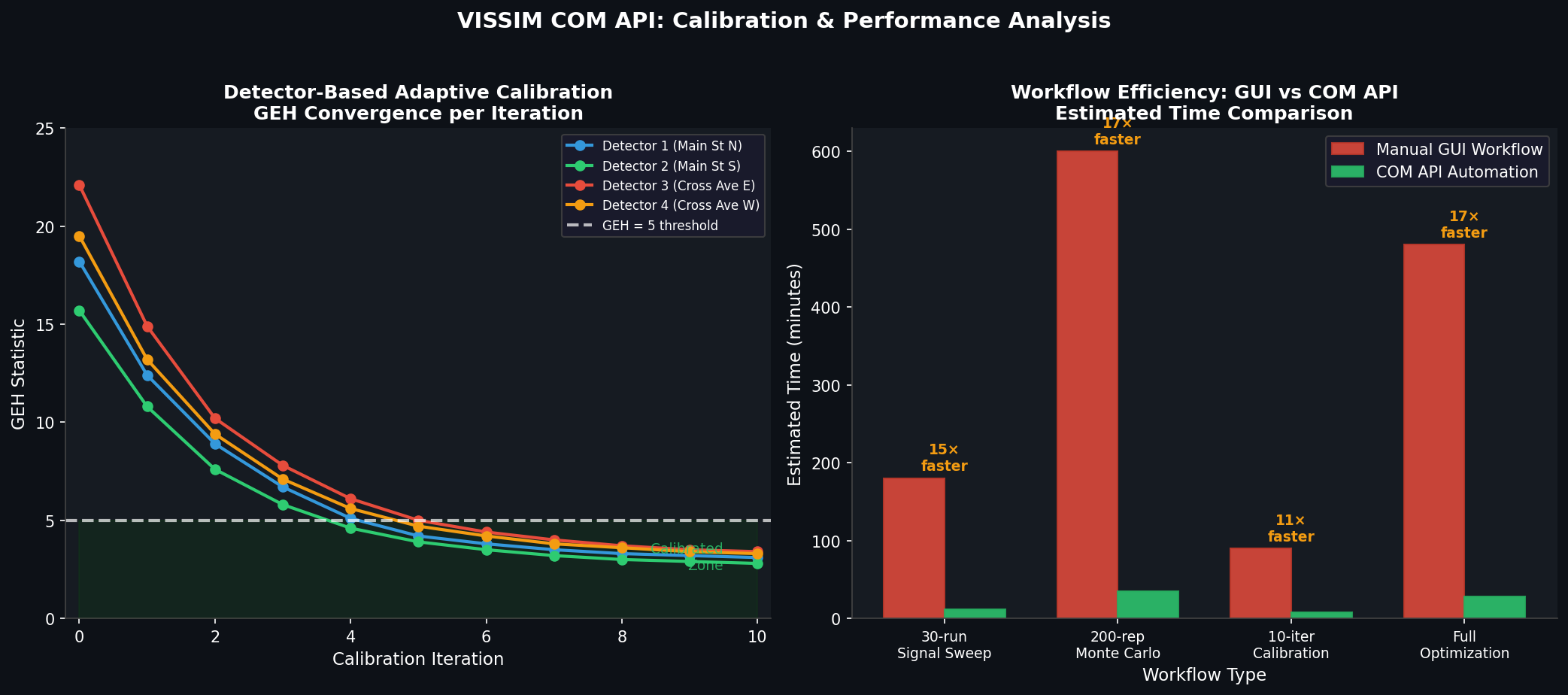
Field loop-detector counts can be fed back into the model in real time (or post-processed) to auto-calibrate vehicle input volumes. The COM API exposes detector objects whose Flows attribute returns simulated counts that can be compared against observed data, and a simple proportional controller can close the loop:

detectors = vissim.Net.DataCollectionMeasurements
for dc in detectors:
    sim_flow = dc.AttValue("Vehs(Current,Last,All)")
    obs_flow = field_counts[dc.AttValue("No")]   # from your field database
    ratio = obs_flow / max(sim_flow, 1)
    # Adjust upstream vehicle input proportionally
    upstream_vi = get_upstream_input(dc)
    upstream_vi.SetAttValue("Volume(1)", upstream_vi.AttValue("Volume(1)") * ratio)

Iterating this loop to convergence (typically 5–10 passes) yields a calibrated model that matches observed counts within the ±15 % GEH threshold recommended by the UK Highways Agency and widely adopted internationally.

Performance Considerations

• Headless mode: Set vissim.Graphics.CurrentNetworkWindow.SetAttValue("QuickMode", 1) to suppress rendering and cut run times by 30–50 %.
• Parallel replications: Launch multiple VISSIM COM instances on separate cores using Python's multiprocessing module; each instance loads its own copy of the network file.
• Result caching: Use VISSIM's built-in SQLite result database (*.fzp) rather than polling attributes after every time step—batch reads are far more efficient.

Integration with External Optimization Frameworks

The COM API's language-agnostic nature means VISSIM can serve as the simulation engine inside frameworks such as:

• Optuna or Ax (Bayesian optimization) for signal timing or ramp metering parameter search
• SUMO-TraCI parity workflows where teams maintain both open-source and commercial models
• Digital twin platforms (e.g., Bentley iTwin, Autodesk Tandem) via REST microservices that wrap the COM calls

Further Resources

• PTV VISSIM COM Interface Manual — shipped with each installation; also available via PTV's customer portal
• PTV Developer Community — active forum with COM API examples and troubleshooting threads
• FHWA Traffic Analysis Toolbox Volume III — guidance on calibration standards and acceptable error thresholds
• pywin32 documentation — Python-to-COM bridge library

Mastering the VISSIM COM API transforms the tool from a point-and-click simulator into a programmable simulation engine that integrates cleanly with modern data science and optimization workflows—an essential skill for any transportation engineer working at scale.