FEniCSx UFL Form Language: Expressing Variational Problems for Automated PDE Solving

The FEniCS Project's next-generation platform, FEniCSx, has redefined how engineers and scientists express and solve partial differential equations (PDEs) computationally. At its core lies the Unified Form Language (UFL) — a domain-specific language embedded in Python that lets practitioners write variational formulations almost exactly as they appear in textbooks, while the framework automatically generates optimized finite element assembly code. This article examines UFL's capabilities, workflow, and best practices for intermediate-level users tackling real-world PDE problems.

What Is FEniCSx and UFL?

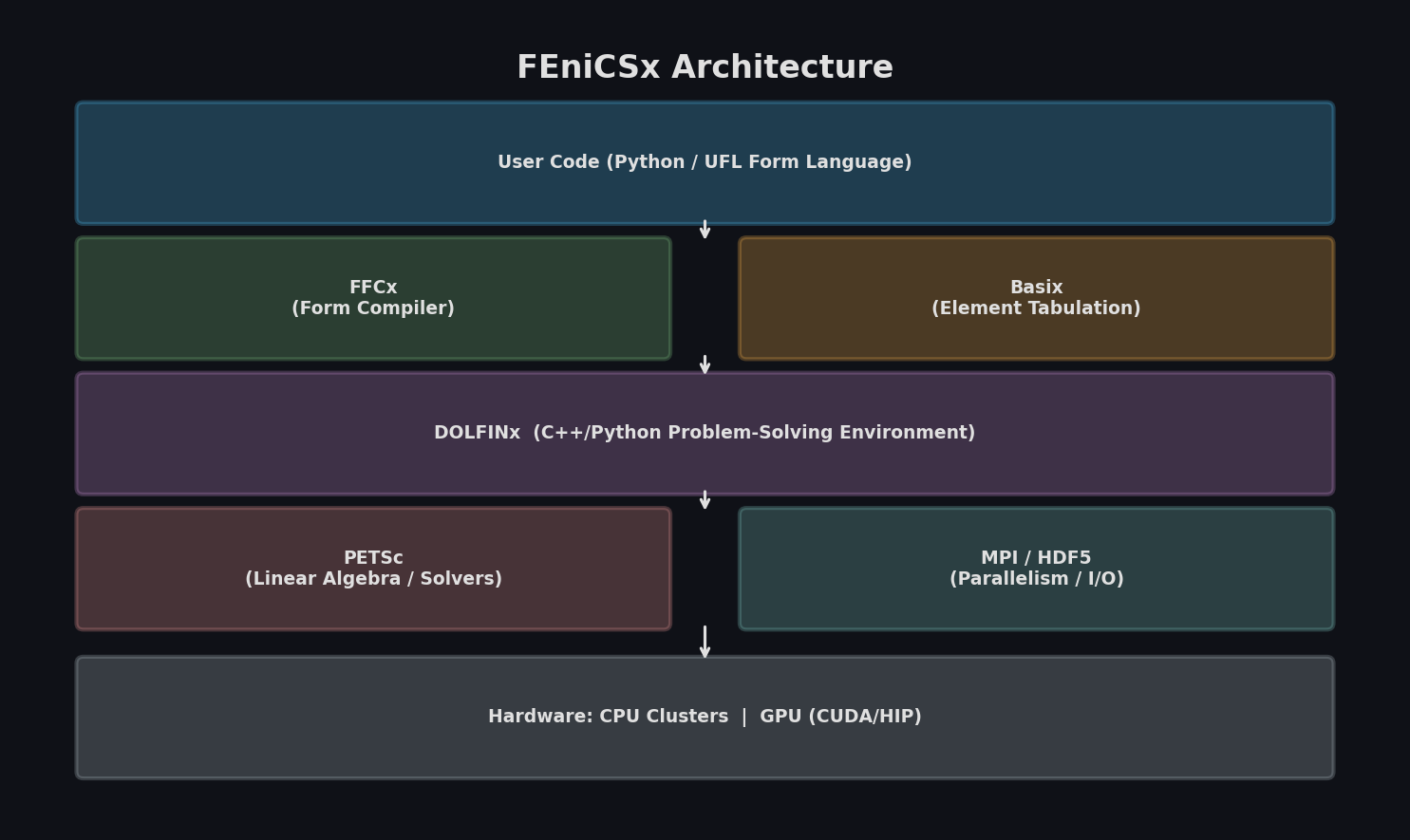
FEniCSx is the modernized successor to the original FEniCS library, rebuilt from the ground up with a cleaner architecture, improved parallelism via MPI, and tighter integration with PETSc for scalable linear algebra. The platform comprises four main components:

• UFL — the symbolic form language for expressing weak formulations
• FFCx — the FEniCS Form Compiler that translates UFL expressions into optimized C kernels
• DOLFINx — the C++/Python problem-solving environment that manages meshes, function spaces, and solvers
• Basix — the finite element definition library providing tabulation of basis functions

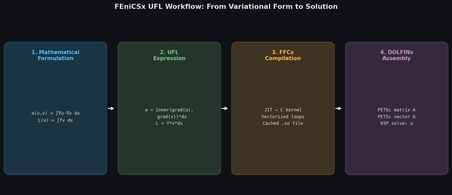
UFL's design philosophy is that the mathematical statement of a problem should be the program. A Poisson equation, for instance, is expressed as:

from dolfinx import mesh, fem
from dolfinx.fem import functionspace
from ufl import TrialFunction, TestFunction, dx, grad, inner
import numpy as np

# Create mesh and function space
domain = mesh.create_unit_square(MPI.COMM_WORLD, 32, 32)
V = functionspace(domain, ("Lagrange", 1))

u = TrialFunction(V)
v = TestFunction(V)

# Bilinear and linear forms — identical to the mathematical notation
a = inner(grad(u), grad(v)) * dx
L = inner(fem.Constant(domain, 1.0), v) * dx

This near-mathematical syntax dramatically reduces the gap between formulation and implementation, minimizing transcription errors that plague lower-level FEM codes.

Key UFL Capabilities for Engineering Problems

1. Arbitrary-Order Elements and Mixed Formulations

UFL supports the full Periodic Table of Finite Elements, including Lagrange, Nédélec, Raviart-Thomas, and Discontinuous Galerkin families. Mixed formulations — essential for incompressible flow (Taylor-Hood elements) or coupled thermo-mechanical problems — are expressed naturally:

from basix.ufl import element, mixed_element

P2 = element("Lagrange", domain.topology.cell_name(), 2)
P1 = element("Lagrange", domain.topology.cell_name(), 1)
TH = mixed_element([P2, P2, P1])  # Taylor-Hood for Stokes flow
W = functionspace(domain, TH)

2. Nonlinear Problems via Automatic Differentiation

UFL's symbolic differentiation engine enables automatic linearization of nonlinear residuals. For a hyperelastic solid mechanics problem, the Jacobian is derived symbolically:

from ufl import derivative, variable, diff

# Neo-Hookean strain energy density
F = Identity(3) + grad(u)
C = F.T * F
Ic = tr(C)
J = det(F)
psi = (mu/2) * (Ic - 3) - mu * ln(J) + (lmbda/2) * (ln(J))**2

# Residual and Jacobian — Jacobian computed automatically
Pi = psi * dx
F_form = derivative(Pi, u, v)
J_form = derivative(F_form, u, du)

This eliminates the error-prone manual derivation of tangent stiffness matrices, a common source of bugs in custom FEM codes.

3. Multiphysics Coupling

UFL handles coupled systems by allowing forms to reference multiple function spaces. A coupled heat-fluid problem can share solution fields across forms, with DOLFINx managing the assembly into block-structured matrices compatible with PETSc's PCFIELDSPLIT preconditioner for efficient iterative solving.

4. Spatially Varying Coefficients and Expressions

Material heterogeneity is expressed through UFL Coefficient objects interpolated onto function spaces, or via Expression objects that map Python/NumPy functions to DOLFINx-compatible representations. This supports realistic material models with spatially varying Young's modulus, thermal conductivity, or permeability fields derived from imaging data.

Performance and Scalability

FFCx compiles UFL forms to C code using TSFC (Two-Stage Form Compiler) technology, generating cell kernels that are JIT-compiled and cached. On modern hardware:

• Single-node performance: DOLFINx achieves near-peak FLOP rates for assembly through vectorized cell kernels
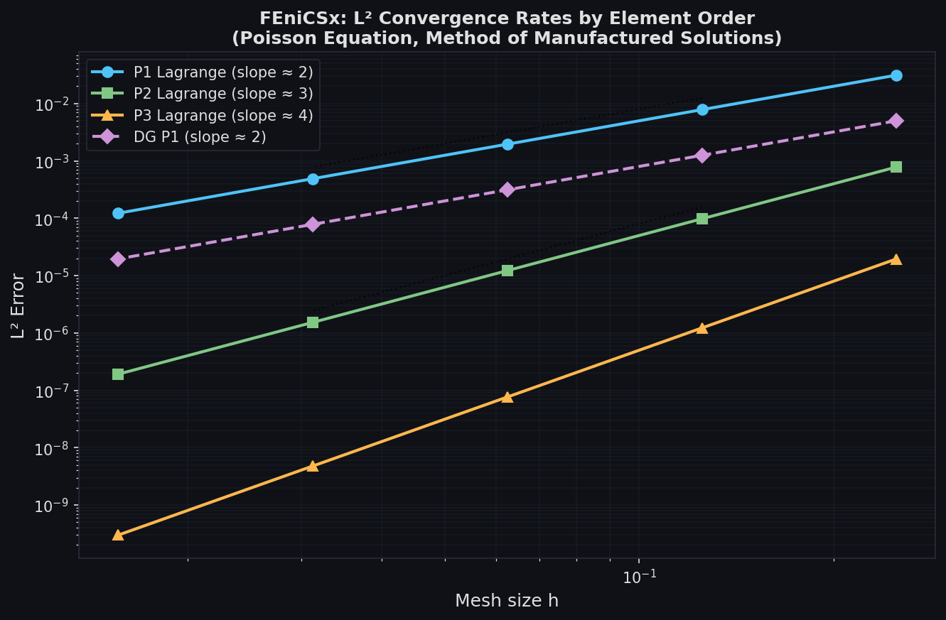
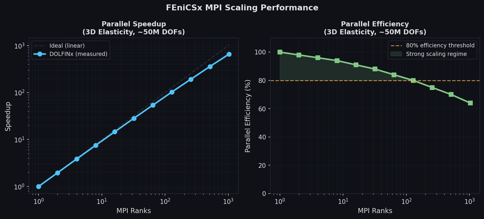
• Parallel scaling: MPI-based domain decomposition scales to thousands of cores on HPC clusters; the FEniCS benchmarking suite demonstrates near-linear scaling to 4,096 MPI ranks for standard elliptic problems
• GPU acceleration: Experimental support via DOLFINX-GPU targets NVIDIA and AMD GPUs through PETSc's CUDA/HIP backends

Practical Workflow: From Geometry to Results

A typical FEniCSx workflow for an engineering simulation proceeds as:

1. Mesh generation: Import from Gmsh (.msh format) using dolfinx.io.gmshio, or generate structured meshes with built-in utilities
2. Boundary condition specification: Use dolfinx.fem.dirichletbc with geometric locators or mesh tags from Gmsh physical groups
3. Form assembly: dolfinx.fem.petsc.assemble_matrix and assemble_vector populate PETSc data structures
4. Solving: Configure PETSc KSP/SNES solvers directly, or use DOLFINx's LinearProblem / NonlinearProblem convenience wrappers
5. Post-processing: Export to ParaView via XDMF/HDF5 using dolfinx.io.XDMFFile

Best Practices and Common Pitfalls

Use physical groups from Gmsh: Tag boundaries and subdomains in Gmsh before import. DOLFINx reads these as MeshTags, enabling clean boundary condition and subdomain integral specification without fragile coordinate-based selection.

Cache compiled forms: FFCx JIT compilation occurs on first run. In production workflows, pre-compile forms with ffcx CLI and import the generated C code to eliminate startup overhead in parameter sweeps.

Choose solvers deliberately: The default direct solver (MUMPS via PETSc) works well for problems up to ~10M DOFs. For larger systems, configure algebraic multigrid (HYPRE BoomerAMG or ML) through PETSc options:

solver.ksp_type = "cg"
solver.pc_type = "hypre"
solver.pc_hypre_type = "boomeramg"

Validate with the Method of Manufactured Solutions (MMS): UFL's symbolic nature makes MMS straightforward — define an exact solution, compute the corresponding source term symbolically, and verify convergence rates match theoretical predictions.

When to Choose FEniCSx

FEniCSx excels when:

• The governing equations are non-standard or research-level, requiring custom weak formulations
• Rapid prototyping of new physics models is needed without sacrificing performance
• Open-source, reproducible, and auditable simulation pipelines are required
• Integration with Python's scientific ecosystem (NumPy, SciPy, PyTorch for ML-augmented simulations) is valuable

Commercial alternatives like ANSYS Mechanical or COMSOL Multiphysics offer superior GUI workflows and pre-built physics modules for standard problems. FEniCSx's advantage is flexibility and programmability for novel formulations.

Further Resources

• FEniCSx Documentation — official API reference and tutorials
• FEniCS Discourse Forum — active community support
• Numerical Tours of Computational Mechanics — advanced tutorial collection
• Baratta et al. (2023), "DOLFINx: The next generation FEniCS problem solving environment" — reference paper

FEniCSx represents a mature, production-ready platform for automated finite element computing. Its UFL form language bridges the gap between mathematical rigor and computational efficiency, making it an indispensable tool for researchers and engineers working at the frontier of computational mechanics and multiphysics simulation.