Implementing GARCH Models for Volatility Forecasting in Financial Simulations

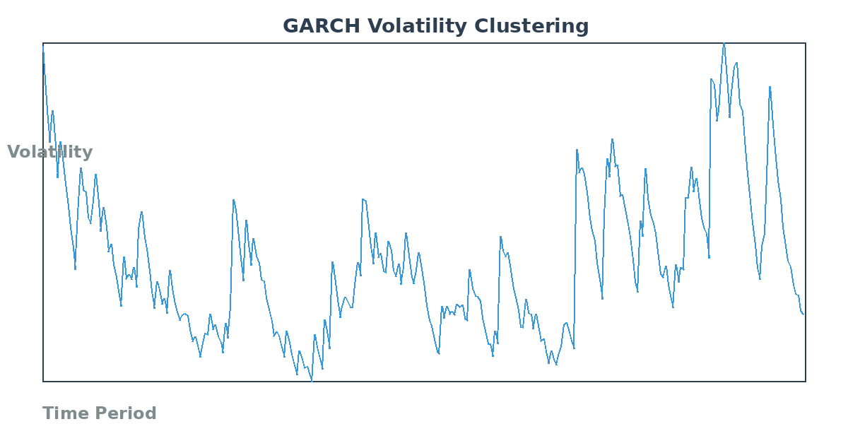
Financial market volatility is not constant—it clusters, spikes during crises, and exhibits mean-reverting behavior. Traditional simulation approaches that assume constant volatility fail to capture these critical dynamics, leading to underestimated risk and poor hedging strategies. Generalized Autoregressive Conditional Heteroskedasticity (GARCH) models provide a robust framework for modeling time-varying volatility, making them essential tools for realistic financial simulations.

Understanding GARCH Model Architecture

GARCH models extend the basic ARCH framework by incorporating lagged conditional variances alongside squared residuals. The standard GARCH(1,1) specification—the most widely used variant—models conditional variance as:

σ²ₜ = ω + α·ε²ₜ₋₁ + β·σ²ₜ₋₁

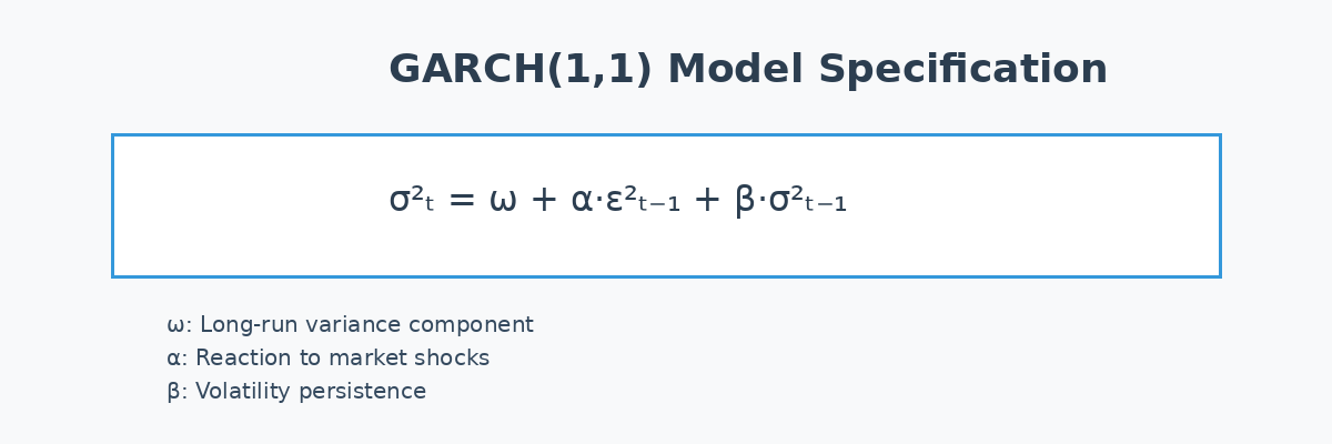
where ω represents the long-run variance component, α captures the reaction to market shocks, and β measures volatility persistence. The sum α + β determines mean reversion speed; values approaching unity indicate high persistence, characteristic of financial time series. This parsimonious structure captures volatility clustering while remaining computationally tractable for large-scale simulations.

Implementation Strategies for Simulation Workflows

Integrating GARCH models into financial simulations requires careful attention to parameter estimation and forecast generation. Maximum likelihood estimation (MLE) remains the standard approach, though quasi-maximum likelihood (QMLE) offers robustness when return distributions deviate from normality. For simulation purposes, practitioners should:

Calibrate on rolling windows: Use 250-500 day estimation windows to balance parameter stability with adaptability to regime changes. Re-estimate parameters quarterly or when volatility regimes shift significantly.

Generate multi-step forecasts: GARCH variance forecasts converge to unconditional variance as the horizon extends. For h-step ahead forecasts, the GARCH(1,1) variance follows: σ²ₜ₊ₕ = σ² + (α+β)ʰ·(σ²ₜ - σ²), where σ² represents long-run variance.

Simulate return paths: Draw standardized innovations from the appropriate distribution (Student-t for fat tails, skewed-t for asymmetry), then scale by forecasted conditional standard deviations to generate realistic price paths.

Advanced Extensions for Specific Applications

Several GARCH variants address specialized simulation requirements. The EGARCH model captures leverage effects where negative returns increase volatility more than positive returns—critical for equity simulations. The GJR-GARCH provides a simpler asymmetric specification through threshold parameters. For multi-asset portfolios, multivariate GARCH models like DCC-GARCH (Dynamic Conditional Correlation) allow time-varying correlations, essential for realistic portfolio stress testing.

Component GARCH models decompose volatility into transitory and permanent components, useful for separating short-term market noise from structural volatility shifts. This proves valuable in scenario analysis where you need to distinguish temporary shocks from regime changes.

Practical Considerations and Validation

GARCH model performance depends critically on proper specification testing. Standardized residuals should exhibit no remaining autocorrelation in squared values—verify using Ljung-Box tests on squared standardized residuals. For simulation validation, compare generated volatility distributions against historical volatility clustering patterns and ensure simulated extreme events occur at realistic frequencies.

Computational efficiency matters for large-scale applications. Modern implementations leverage GPU acceleration for parallel simulation paths, while analytical variance forecasts avoid recursive computation bottlenecks. Python's arch package and R's rugarch provide production-ready implementations with extensive diagnostic tools.

Integration with Risk Management Frameworks

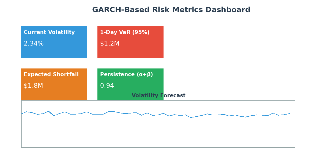
GARCH-based simulations enhance Value-at-Risk (VaR) and Expected Shortfall (ES) calculations by incorporating volatility dynamics. Static volatility assumptions systematically underestimate risk during volatile periods and overestimate during calm markets. GARCH-filtered simulations produce time-varying risk metrics that adapt to current market conditions, improving capital allocation and regulatory compliance.

For stress testing, combine GARCH volatility forecasts with scenario-specific shock parameters. This hybrid approach maintains realistic volatility dynamics while exploring tail events beyond historical experience. Backtesting should compare GARCH-based risk metrics against realized outcomes across multiple market cycles to validate model performance.

Further Resources

For comprehensive GARCH theory and applications, consult Engle's original work and Bollerslev's extensions in the Journal of Econometrics. The arch Python package documentation provides detailed implementation guidance: https://arch.readthedocs.io/. For multivariate extensions, Engle's DCC-GARCH paper remains the definitive reference. Practitioners should also review regulatory guidance on volatility modeling from Basel Committee publications for compliance considerations.

GARCH models represent a mature, well-validated approach to volatility forecasting that significantly improves financial simulation realism. Their computational efficiency and theoretical foundation make them indispensable for modern quantitative risk management and derivative pricing applications.