
Inventory Policy Optimization in AnyLogic: Simulating (s, S) and (r, Q) Replenishment Strategies
Inventory management sits at the intersection of cost control and service-level assurance. Choosing the wrong replenishment policy—or calibrating it with static spreadsheet models—can lock millions of dollars in excess stock or, conversely, trigger costly stockouts. AnyLogic's multi-method simulation environment gives supply chain engineers a rigorous, data-driven path to compare and tune inventory policies before committing to live operations.
Why Simulation Beats Analytical Formulas Alone
Classical inventory theory provides closed-form solutions for the Economic Order Quantity (EOQ) and reorder-point calculations, but these formulas rest on assumptions that rarely hold in practice: constant demand, deterministic lead times, and no supply disruptions. Real distribution networks exhibit:
- Lumpy, seasonal demand driven by promotions, weather, or product life cycles
- Stochastic lead times from suppliers with variable production and transit schedules
- Correlated stockouts across SKUs sharing warehouse space or transportation capacity
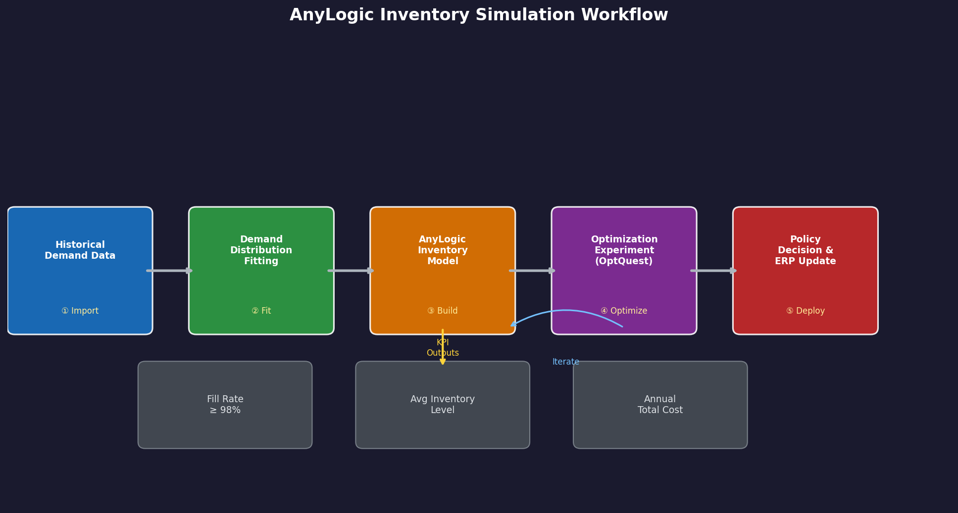
AnyLogic's discrete-event and agent-based layers let you model all of these dynamics simultaneously, running thousands of replications to build statistically robust confidence intervals around KPIs such as fill rate, average inventory level, and total holding plus ordering cost.

Modeling the (s, S) Policy
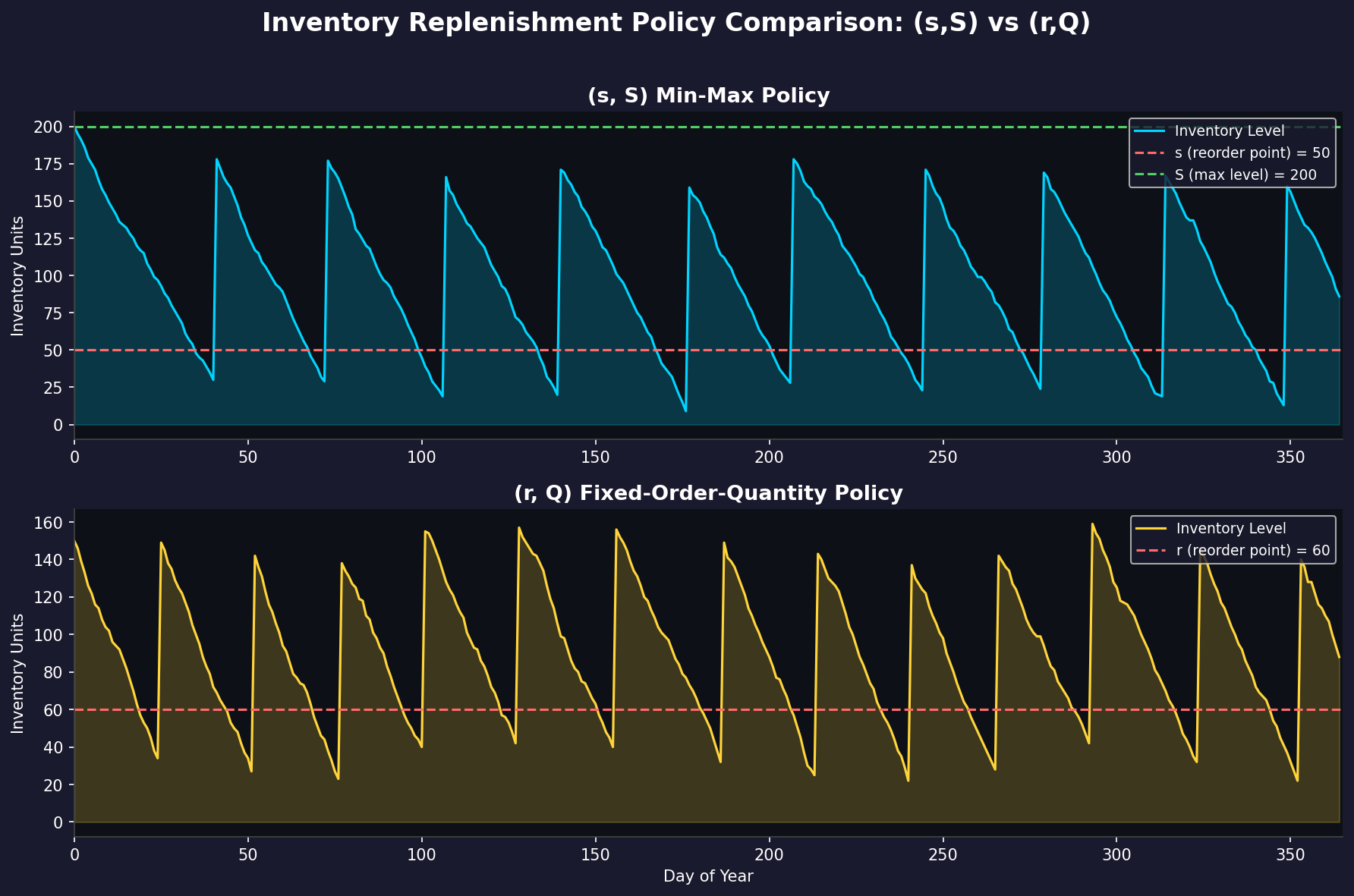
The (s, S) (min-max) policy triggers a replenishment order whenever on-hand inventory falls to or below the reorder point s, bringing stock up to the order-up-to level S. In AnyLogic, this is implemented using the Inventory object from the Process Modeling Library combined with a SelectOutput block that routes demand to either on-hand stock or a backorder queue.
// AnyLogic Java action on InventoryLevel change
if (inventoryLevel <= s_reorderPoint) {
    double orderQty = S_maxLevel - inventoryLevel;
    sendOrder(orderQty);
}
Key parameters to expose as experiment variables include s_reorderPoint, S_maxLevel, and leadTimeMean / leadTimeStd. Wrapping the model in an Optimization experiment (using the built-in OptQuest engine) allows AnyLogic to search the parameter space automatically, minimizing total cost subject to a fill-rate constraint (e.g., ≥ 98%).
Modeling the (r, Q) Policy
The (r, Q) (continuous-review, fixed-order-quantity) policy places a fixed order of size Q whenever inventory drops to the reorder point r. This policy is common in manufacturing environments where supplier contracts specify fixed lot sizes or where ordering costs are high relative to holding costs.
In AnyLogic, the distinction from (s, S) is subtle but important: Q is constant regardless of current inventory depth, whereas in (s, S) the order quantity varies. Implement this by replacing the dynamic orderQty calculation with a fixed constant:
if (inventoryLevel <= r_reorderPoint) {
    sendOrder(Q_fixedOrderQty);
}
Running both policies side-by-side in a Comparison experiment with identical demand traces (using a seeded random stream) produces apples-to-apples cost and service-level comparisons.
Setting Up the Simulation Experiment
A well-structured AnyLogic inventory model should include:
- Demand generator — Use an
EventTimeoutblock with an inter-arrival time drawn from a fitted distribution (e.g., Negative Binomial for lumpy demand). Import historical demand data via Excel or a database connector. - Supplier lead time — Model as a
delayblock with a triangular or log-normal distribution parameterized from supplier scorecards. - Warehouse capacity constraint — Add a
ResourcePoolrepresenting physical storage slots to capture the cost of overflow. - KPI collectors — Use
TimeMeasureStart/Endblocks andDataSetobjects to track fill rate, average cycle stock, and safety stock levels across replications. - Warm-up period — Set a warm-up of at least 30 days (or one demand cycle) to eliminate initialization bias before collecting statistics.
Interpreting Results and Policy Selection
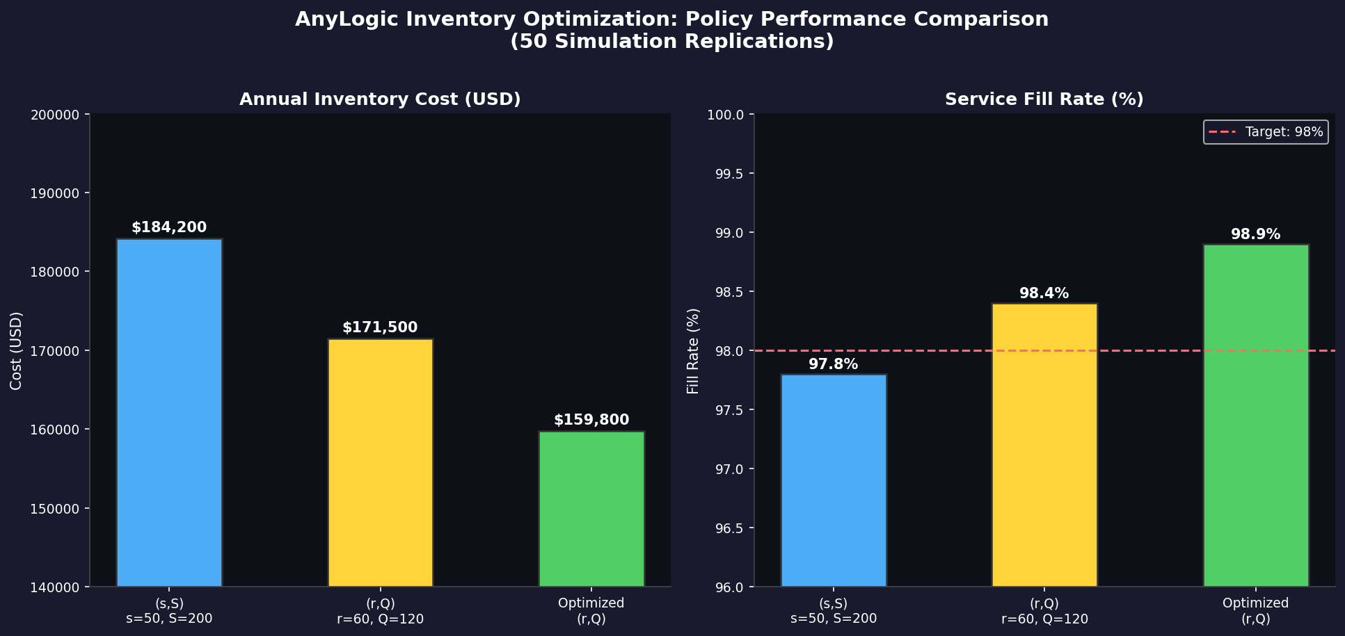
After running 50–100 replications per policy configuration, AnyLogic's Statistics panel provides mean, standard deviation, and confidence intervals for each KPI. A typical output comparison might look like:
| Policy | Avg. Inventory (units) | Fill Rate | Annual Cost (USD) |
|---|---|---|---|
| (s, S) s=50, S=200 | 112 | 97.8% | $184,200 |
| (r, Q) r=60, Q=120 | 98 | 98.4% | $171,500 |
| Optimized (r, Q) | 87 | 98.9% | $159,800 |
The optimized (r, Q) policy in this example reduces annual cost by 13% while improving fill rate—an outcome that static EOQ formulas would not have predicted because they ignore lead-time variability.
Integration with Real-Time Data
AnyLogic supports database connectivity via JDBC, enabling the model to pull live inventory snapshots from an ERP system (SAP, Oracle, or Microsoft Dynamics) at the start of each simulation run. This transforms the model from a one-time design tool into a rolling decision-support system: planners re-run the simulation weekly with updated demand forecasts and supplier lead-time data to recalibrate reorder points dynamically.
For organizations pursuing a digital twin strategy, AnyLogic's REST API and Cloud platform allow the inventory model to be embedded in a web dashboard, giving supply chain managers on-demand scenario analysis without requiring AnyLogic licenses on every desktop.
Best Practices and Pitfalls
- Fit demand distributions carefully. Using a Normal distribution for lumpy demand underestimates tail risk. Use the AnyLogic Data Fitting tool or an external tool like EasyFit to select the best-fit distribution before building the model.
- Account for review period latency. Even in continuous-review systems, ERP batch processing introduces effective review periods of hours. Model this explicitly to avoid overly optimistic fill-rate predictions.
- Validate against historical data. Run the model over a historical period with known outcomes and compare simulated fill rates and inventory levels to actuals before using the model for forward-looking decisions.
- Sensitivity analysis is mandatory. Use AnyLogic's Parameter Variation experiment to understand how sensitive your chosen policy is to demand forecast errors—a policy that looks optimal under the base forecast may perform poorly under a 20% demand surge.
Further Resources
- AnyLogic Inventory Simulation Tutorial — Official use-case library with downloadable model examples
- AnyLogic Help: Process Modeling Library — Full API reference for inventory and queue objects
- APICS CPIM Body of Knowledge — Foundational inventory management theory underlying simulation model design
- Silver, Pyke & Thomas: Inventory Management and Production Planning and Scheduling — Authoritative reference for (s, S) and (r, Q) policy mathematics
Simulation-driven inventory optimization is no longer a luxury reserved for Fortune 500 supply chains. With AnyLogic's accessible modeling environment and built-in optimization engine, mid-market manufacturers and distributors can achieve the same analytical rigor—turning inventory policy decisions from educated guesses into statistically defensible engineering choices.