LS-DYNA Implicit Solver: Best Practices for Nonlinear Structural Analysis

LS-DYNA is widely recognized for its explicit dynamics capabilities, but its implicit solver is an equally powerful—and often underutilized—tool for nonlinear structural analysis. When engineers need to study quasi-static loading, springback in metal forming, or structural response under slowly applied loads, the implicit solver offers superior accuracy and computational efficiency compared to running explicit analyses with artificially shortened time scales. This article examines the key features, configuration strategies, and best practices for leveraging LS-DYNA's implicit solver in demanding nonlinear structural problems.

Why Choose Implicit Over Explicit?

The fundamental difference between implicit and explicit time integration lies in how each method advances the solution in time. Explicit methods compute the state at the next time step directly from the current state—no system of equations needs to be solved—but stability requires extremely small time steps (on the order of microseconds for typical metal parts). Implicit methods solve a system of equations at each step, allowing much larger time increments and making them ideal for:

• Quasi-static analyses (press forming, bolted joint preload, assembly fit-up)
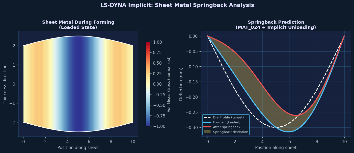
• Springback prediction following sheet metal stamping
• Creep and relaxation studies under sustained loading
• Eigenvalue and modal analyses for natural frequency extraction
• Nonlinear buckling under compressive loads

For these problem classes, running an explicit analysis requires mass scaling or artificially high loading rates—both of which introduce inertial artifacts that corrupt results. The implicit solver eliminates this concern entirely.

Activating and Configuring the Implicit Solver

The implicit solver is activated in LS-DYNA through the *CONTROL_IMPLICIT_GENERAL keyword. The most critical parameters are:

*CONTROL_IMPLICIT_GENERAL
$ IMFLAG  DT0    IMFORM  NSBS  IGS  CNSTN  FORM  ZERO_V
       1  0.1         2     1    2      0     0       0

• IMFLAG = 1 switches the solver to implicit mode.
• DT0 sets the initial time step size. For quasi-static analyses, this is typically a fraction of the total simulation time.
• IMFORM = 2 selects the updated Lagrangian formulation, which is appropriate for large-deformation problems.

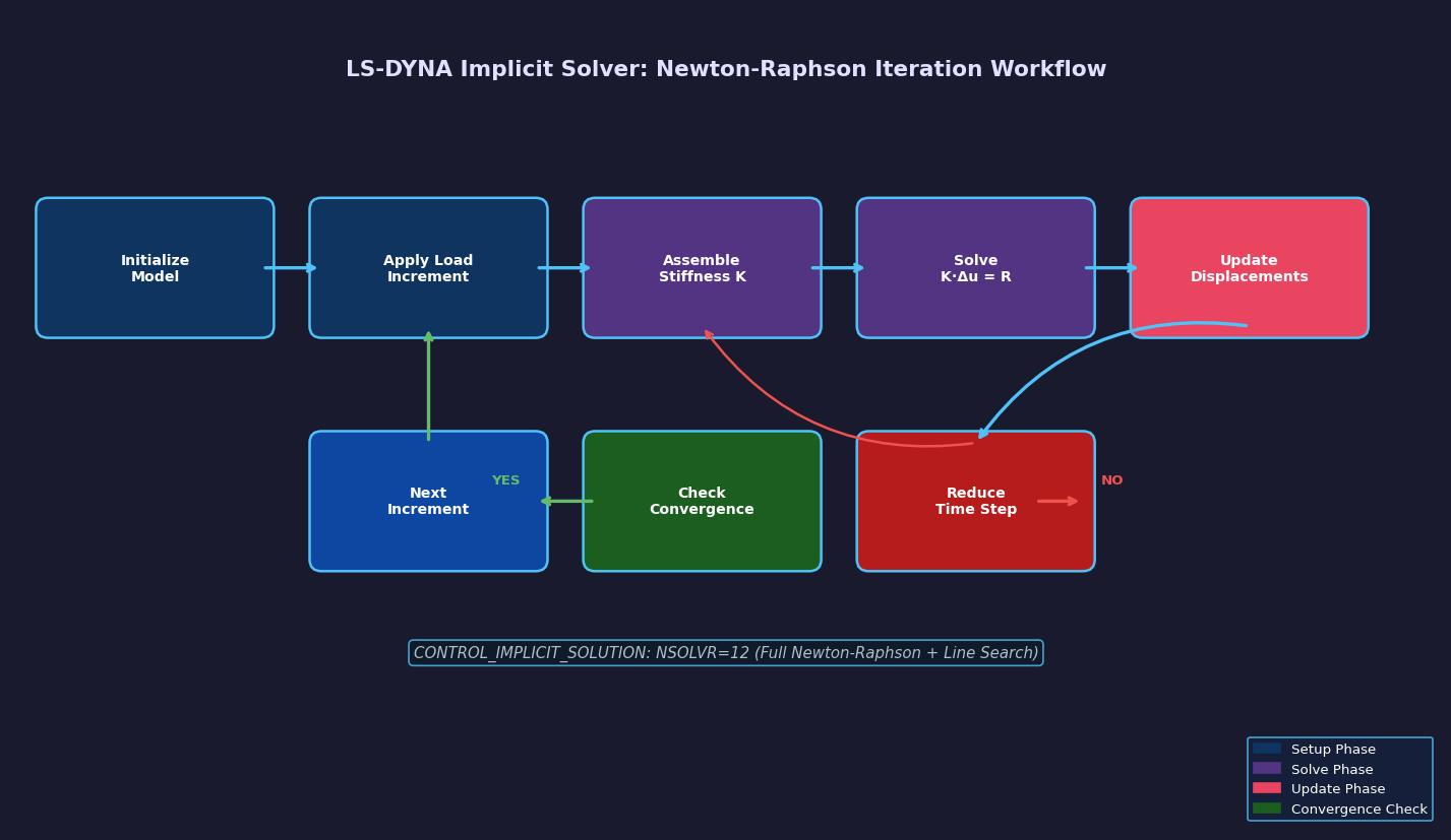
For nonlinear problems, Newton-Raphson iteration is controlled via *CONTROL_IMPLICIT_SOLUTION:

*CONTROL_IMPLICIT_SOLUTION
$ NSOLVR  ILIMIT  MAXREF  DCTOL   ECTOL   RCTOL   LSTOL  ABSTOL
       12      11      15  0.001  0.01    1.0E-10   0.9   1.0E-10

Setting NSOLVR = 12 enables the full Newton-Raphson method with line search, which provides robust convergence for highly nonlinear contact and material problems. The displacement convergence tolerance DCTOL = 0.001 (0.1%) is appropriate for most structural analyses; tighter tolerances may be needed for contact-dominated problems.

Handling Nonlinear Contact in Implicit Analyses

Contact is one of the most challenging aspects of implicit nonlinear analysis. LS-DYNA's *CONTACT_AUTOMATIC_SURFACE_TO_SURFACE with the SOFT = 2 (segment-based penalty) option is recommended for implicit analyses because it provides better convergence behavior than the default node-to-segment formulation.

Key contact settings for implicit stability:

• SOFT = 2: Segment-based contact with area-weighted penalty—reduces oscillations at contact interfaces.
• PENOPT = 5: Uses the minimum of master/slave stiffness for penalty calculation, preventing over-constraint.
• IGNORE = 2: Allows initial penetrations to be resolved gradually, avoiding sudden force spikes at the first step.

For problems with significant sliding (e.g., deep-draw forming), enabling automatic contact stiffness scaling (SHLTHK = 2) helps maintain convergence as contact patches evolve.

Material Nonlinearity: Plasticity and Large Strains

LS-DYNA's implicit solver supports the full library of material models, but some are better suited to implicit analysis than others. For metal plasticity, *MAT_024 (Piecewise Linear Plasticity) and *MAT_036 (Barlat 3-Parameter Plasticity) are well-tested with the implicit solver and support consistent tangent moduli—essential for quadratic convergence in Newton-Raphson iteration.

When defining hardening curves, ensure the true stress–true strain data extends well beyond the expected strain range. Extrapolation artifacts at the end of the hardening curve are a common source of convergence failures in deep-draw simulations.

For rubber and elastomers, *MAT_077 (Ogden) and *MAT_127 (Arruda-Boyce) provide analytically derived tangent stiffness matrices that significantly improve convergence compared to numerically differentiated alternatives.

Adaptive Time Stepping

LS-DYNA's implicit solver includes automatic time step control via *CONTROL_IMPLICIT_AUTO:

*CONTROL_IMPLICIT_AUTO
$ IAUTO  ITEOPT  ITEWIN  DTMIN   DTMAX   DTEXP  KFAIL  KCYCLE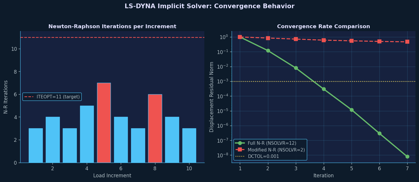
      1      11       5  1.0E-6    0.1     0.0      7       0

• IAUTO = 1 enables automatic time stepping.
• ITEOPT = 11 is the target number of Newton-Raphson iterations per step; the solver increases the time step if convergence is achieved in fewer iterations and reduces it if more are needed.
• KFAIL = 7 allows up to 7 bisections before the analysis terminates, providing a safety net for difficult convergence regions.

This adaptive scheme is particularly valuable for springback analyses, where the unloading phase can involve rapid changes in contact status that require smaller time steps.

Eigenvalue Analysis for Pre-Stressed Structures

One of the most powerful applications of LS-DYNA's implicit solver is performing eigenvalue analyses on pre-stressed structures. By combining an implicit static preload step with a subsequent eigenvalue extraction (*CONTROL_IMPLICIT_EIGENVALUE), engineers can compute natural frequencies of bolted assemblies under realistic clamping loads, turbine blades under centrifugal stress, or pressurized vessels.

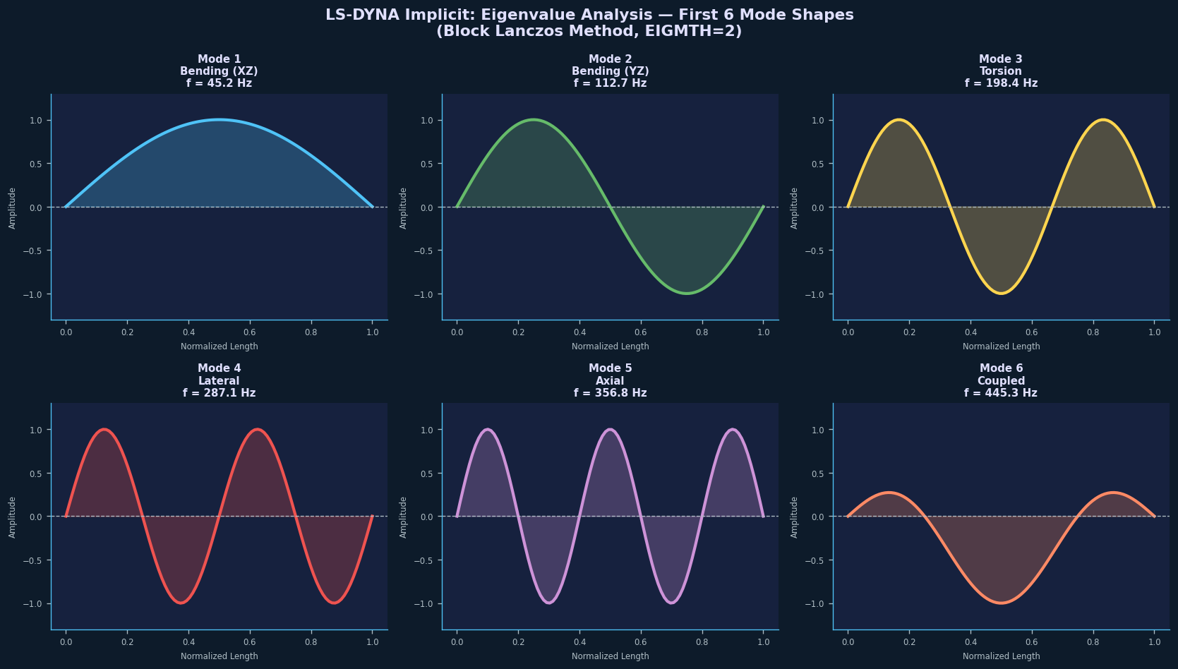
*CONTROL_IMPLICIT_EIGENVALUE
$ NEIG  CENTER  LFLAG  LFTEND  RFLAG  RFTEND  EIGMTH  SHFSCL
    10     0.0      0     0.0      0     0.0       2     0.0

Setting EIGMTH = 2 selects the Block Lanczos method, which is efficient for extracting a moderate number of modes (10–50) from large models.

Practical Workflow Recommendations

1. Start with a coarse mesh to verify contact setup and material behavior before committing to a fine-mesh production run.
2. Use *DATABASE_GLSTAT and *DATABASE_MATSUM to monitor energy balance—a sudden spike in hourglass energy or kinetic energy in a quasi-static analysis signals a convergence problem.
3. *Enable `CONTROL_IMPLICIT_SOLVER` with LSOLVR = 2** (MCGS iterative solver) for models exceeding 500,000 DOF; the direct solver becomes memory-bound at this scale.
4. Archive the d3hsp file after each run—it contains the Newton-Raphson iteration history and is invaluable for diagnosing convergence failures.
5. Validate against a known analytical solution (e.g., a simply supported beam under uniform load) before running complex production models.

Conclusion

LS-DYNA's implicit solver is a mature, production-ready tool for nonlinear structural analysis that complements the software's well-known explicit capabilities. By carefully configuring the Newton-Raphson solver, contact formulations, and adaptive time stepping, engineers can tackle springback, preload, and eigenvalue problems with confidence. The investment in learning the implicit keyword set pays dividends in accuracy and simulation speed for the broad class of quasi-static and low-frequency structural problems that explicit analysis handles poorly.

Further Reading:

• LS-DYNA Keyword User's Manual Vol. I – Implicit Controls
• LSTC Implicit Analysis Best Practices (Livermore Software)
• LS-DYNA Support Forum – Implicit Solver Topics
• ANSYS LS-DYNA Documentation Hub