
PyPSA: Sector-Coupled Energy System Optimization for Net-Zero Planning
PyPSA (Python for Power System Analysis) has evolved well beyond its origins as a power-flow solver into a full-featured, open-source framework for multi-carrier, multi-period energy system optimization. Where tools like pandapower excel at operational AC power-flow studies, PyPSA targets a different problem class: long-run capacity expansion planning across electricity, heat, hydrogen, and gas networks simultaneously. For engineers and researchers designing pathways to net-zero energy systems, PyPSA's sector-coupling capabilities are increasingly indispensable.
What Sets PyPSA Apart
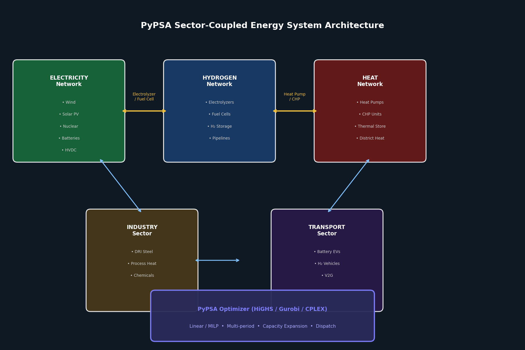
Most power system simulators treat the electricity network in isolation. PyPSA breaks that boundary by representing multiple energy carriers — electricity, gas, hydrogen, heat, liquid fuels — as interconnected networks within a single optimization model. Each carrier has its own buses, lines, and stores; converters (electrolyzers, heat pumps, fuel cells, CHP units) link them. This architecture directly mirrors the physical reality of a decarbonizing energy system where sector coupling is not optional but structural.
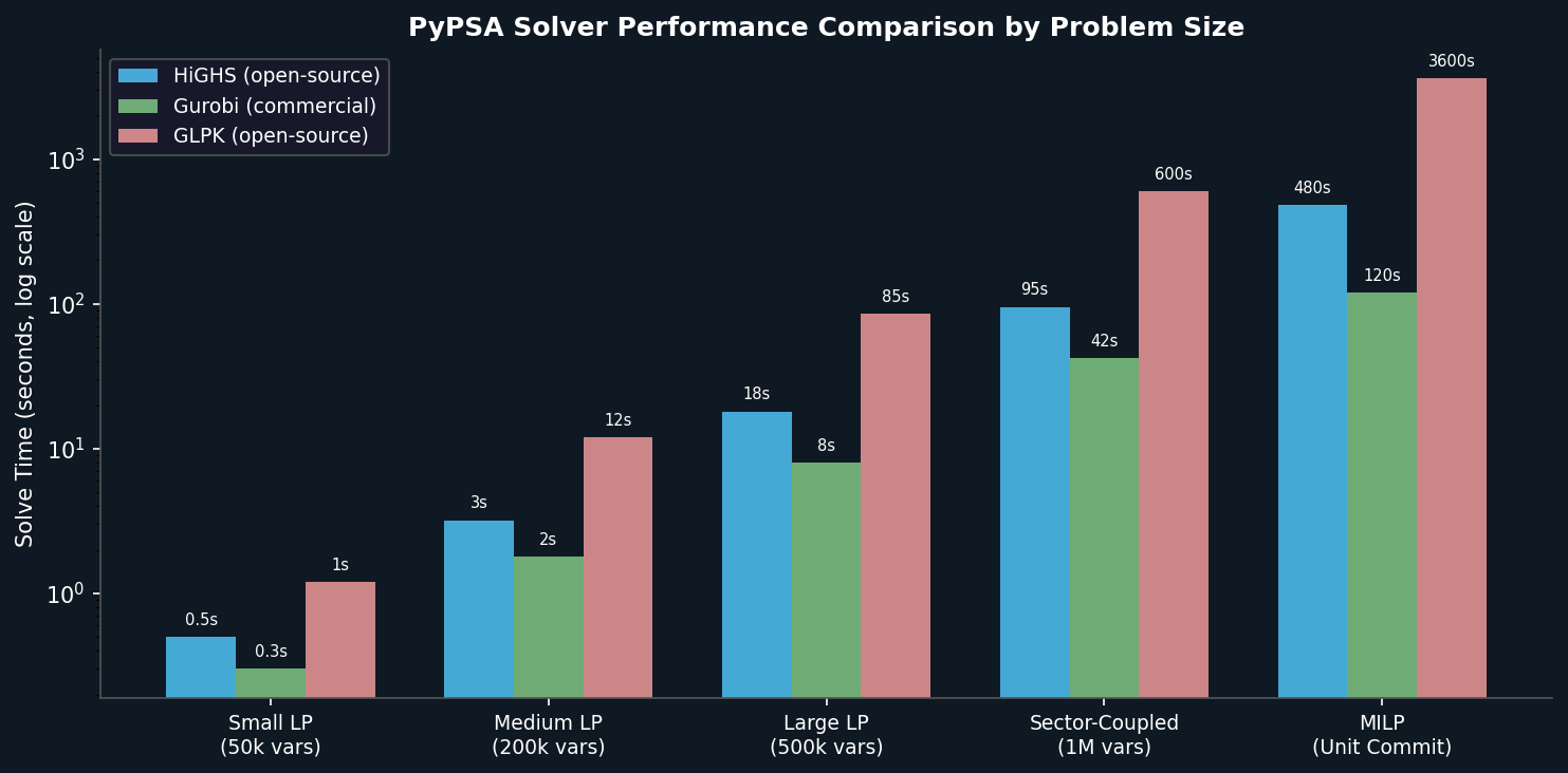
The framework is built on linear and mixed-integer linear programming (MILP), solved via open-source (HiGHS, GLPK) or commercial (Gurobi, CPLEX) backends. The optimization objective is typically total system cost minimization subject to:

- Kirchhoff's voltage laws (linearized DC approximation or full AC)
- Generator capacity limits and ramp rates
- Storage state-of-charge continuity
- CO₂ emission caps or carbon budgets
- Network transmission constraints (N-0 or N-1 security)
Multi-Period Investment Optimization
PyPSA's optimize module (introduced in v0.20, replacing the legacy lopf interface) supports multi-investment-period planning. Engineers can define a sequence of planning horizons (e.g., 2030, 2035, 2040, 2050) with technology cost trajectories, existing asset retirements, and brownfield constraints. The solver simultaneously determines:
- Optimal new capacity for each technology in each period
- Dispatch schedules across representative time slices
- Transmission expansion on AC and DC corridors
This is the same problem class addressed by commercial tools like PLEXOS or TIMES, but PyPSA exposes the full model as a Python object, making it straightforward to inspect, modify, and extend.
import pypsa

n = pypsa.Network()
n.set_snapshots(pd.date_range("2030-01-01", periods=8760, freq="h"))

# Add investment periods
n.investment_periods = [2030, 2040, 2050]
n.investment_period_weightings["years"] = [10, 10, 10]

# Add a wind generator with extendable capacity
n.add("Generator", "offshore_wind",
      bus="DE",
      carrier="wind",
      p_nom_extendable=True,
      capital_cost=1200,   # €/MW/year
      marginal_cost=0,
      p_max_pu=wind_cf_series)

n.optimize(solver_name="highs")
print(n.generators.p_nom_opt)  # Optimal installed capacity per period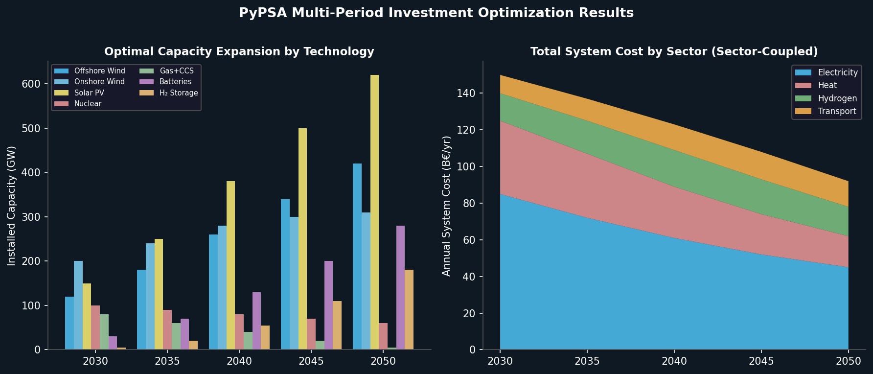
Sector-Coupling Workflow
A typical PyPSA-Eur sector-coupled model (the flagship open dataset built on PyPSA) includes:
| Sector | Components |
|---|---|
| Electricity | Wind, solar PV, nuclear, hydro, batteries, HVDC links |
| Heating | Heat pumps, resistive heaters, district heating networks, thermal stores |
| Hydrogen | Electrolyzers, fuel cells, H₂ pipelines, underground storage |
| Industry | Direct reduced iron (DRI), process heat demands |
| Transport | Battery EVs (V2G), hydrogen fuel-cell vehicles |
The PyPSA-Eur workflow automates data retrieval (ENTSO-E, ERA5 weather, Eurostat demand), network clustering, and scenario runs. A full European model with 181 nodes and 8,760 hourly snapshots can be solved in under 30 minutes on a workstation with HiGHS.
Spatial Network Representation
Unlike energy-system models that treat countries as copper plates, PyPSA supports spatially explicit networks with transmission constraints. The linopt module constructs the LP matrix directly in sparse format, enabling models with tens of thousands of variables to solve efficiently. Engineers can choose between:
- Copper-plate (no transmission limits) — fastest, useful for technology screening
- DC power flow (linearized) — captures congestion, suitable for planning studies
- AC power flow (non-linear) — full physics, used for operational validation
Practical Guidance for Production Studies
Temporal resolution trade-offs: Full 8,760-hour models are computationally expensive for large networks. PyPSA integrates with tsam (time-series aggregation methods) to reduce to 30–100 representative periods while preserving seasonal storage behavior. Validate aggregation error against the full-year baseline before using reduced models for policy decisions.
Solver selection: HiGHS (open-source) handles most LP problems up to ~500k variables efficiently. For MILP unit-commitment problems or very large sector-coupled models, Gurobi provides 5–10× speedups. The linopt interface avoids Pyomo overhead, reducing model build time by 50–80% compared to earlier PyPSA versions.
Uncertainty and scenarios: PyPSA does not natively support stochastic programming, but engineers commonly run Monte Carlo scenario sweeps using Python's multiprocessing or workflow managers like Snakemake (used by PyPSA-Eur). Each scenario is a deterministic LP; results are aggregated post-hoc.
Validation: Cross-check dispatch results against ENTSO-E transparency data or EIA generation statistics. For investment results, compare levelized cost of electricity (LCOE) and capacity factors against published benchmarks (NREL ATB, IRENA cost reports).
When to Choose PyPSA
PyPSA is the right tool when:
- The study requires cross-sector optimization (power + heat + hydrogen)
- Long-run capacity expansion across multiple decades is the primary question
- Full reproducibility and auditability are required (open-source, version-controlled)
- The team is Python-proficient and needs to customize the model
It is less suited for detailed electromagnetic transient studies (use PSCAD or EMTP), real-time operational dispatch with unit-commitment detail (use PLEXOS or SCUC solvers), or protection coordination analysis (use ETAP or CAPE).
Further Resources
- PyPSA Documentation — comprehensive API reference and tutorials
- PyPSA-Eur — open European sector-coupled model
- PyPSA-Earth — global coverage adaptation
- HiGHS Solver — open-source LP/MIP solver used by default
- NREL Annual Technology Baseline — cost data for technology parameterization
- tsam: Time Series Aggregation Module — temporal reduction for large models
PyPSA's combination of rigorous network physics, multi-carrier optimization, and Python-native extensibility makes it one of the most powerful open-source tools available for engineers and researchers working on the energy transition. Its active development community and growing ecosystem of pre-built datasets lower the barrier to entry for production-grade net-zero planning studies.